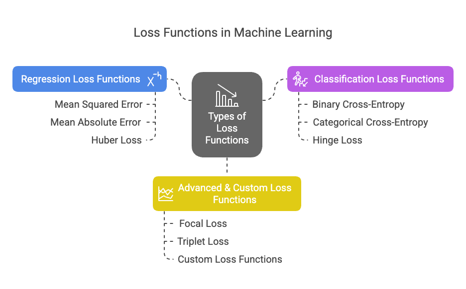
Core Machine Learning Concepts Part 1 - Loss Function
Explore how AI models learn from mistakes and improve over time, using key tools that guide them towards smarter predictions and better decisions.
AI models are like digital brains that learn from data to make decisions or predictions.
A loss function is like a "mistake meter" for AI models. It measures how wrong the model’s predictions are compared to the real answers.
The goal? Minimize this mistake score to make the model smarter.
🍎 Example: Predicting Apple Prices
Let’s say you’re building an AI to predict apple prices:
| Real Price ($) | Model’s Guess ($) | Error (Loss) |
|---|---|---|
| 5 (actual) | 4 (predicted) | 1 (too low) |
| 3 (actual) | 6 (predicted) | 3 (too high) |
The loss function calculates these errors (e.g., Loss = |Real - Guess|) and tells the model:
"Hey, your guesses are off by $1 and $3. Try again!"
A loss function simply measures how wrong a model's predictions are compared to the actual values. It’s like a score that tells the model how much it needs to improve. The goal of training a machine learning model is to minimize this loss, so the model's predictions get as close as possible to the true values.
In simpler terms:
- Small loss → Good predictions
- Large loss → Bad predictions
In machine learning, "loss function" and "cost function" are often used interchangeably, but there's a subtle distinction: the loss function measures the error for a single data point, while the cost function aggregates the loss across an entire dataset or mini-batch.
How Loss Guides Learning (Step-by-Step)
- Model Guesses: Predicts apple prices (e.g., $4, $6).
- Loss Computes Error: Measures how far guesses are from real prices ($5, $3).
- Model Adjusts: Tweaks its math to reduce the loss (e.g., guesses $4.50 next time).
- Repeat: Until loss is as small as possible!
🎯 Why Loss Functions Matter
- Feedback for AI: Like a coach telling a player, "Aim left next time!"
- Optimization: Helps algorithms (e.g., Gradient Descent) adjust the model’s math.
- Task-Specific:
- Predicting prices? Use MSE (punishes big errors).
- Detecting spam? Use Cross-Entropy (works with probabilities).
Understand in detail here:
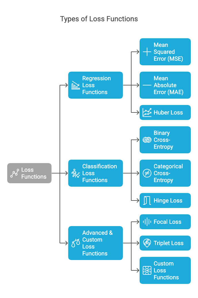
1. Regression Loss Functions (For Predicting Numbers)
A. Mean Squared Error (MSE / L2 Loss)
MSE calculates the average of the squared differences between predicted and actual values. It gives more weight to larger errors, encouraging the model to focus on correcting big mistakes.
Imagine: You're learning to shoot arrows at a target.
- MSE is like a strict coach who hates big mistakes.
- If you miss by 1 inch, it says: "Not bad, but improve."
- If you miss by 5 inches, it screams: "THIS IS UNACCEPTABLE!" (because 5² = 25 penalty).
Where it's used:
- Predicting house prices (big errors cost money!)
- Weather forecasting (small errors matter less than huge ones)
Example:
- Actual temperature: 30°C
- Prediction 1: 28°C → Error = (30-28)² = 4
- Prediction 2: 20°C → Error = (30-20)² = 100 (10x worse!)
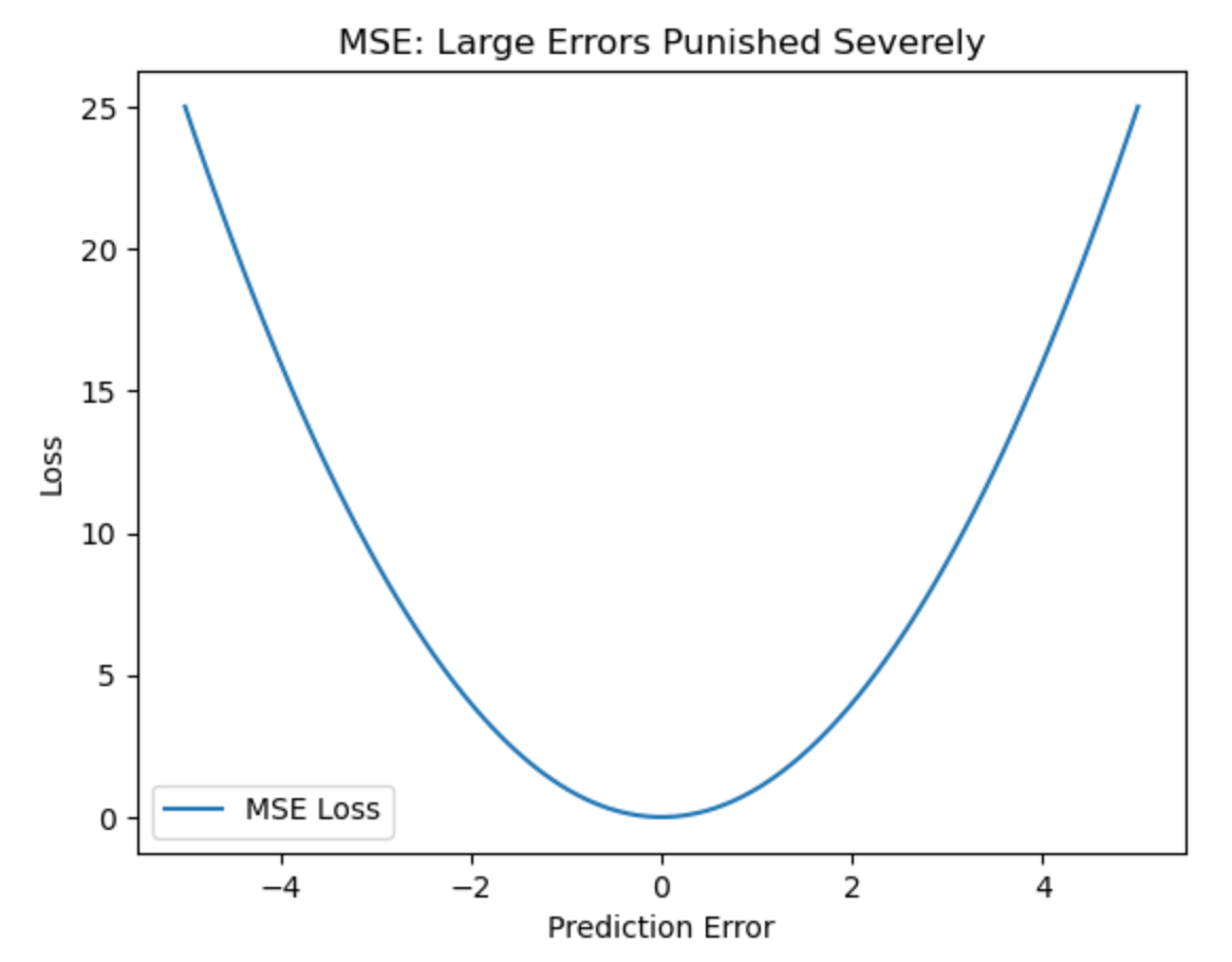
What the graph shows:
- The curve is parabolic - minor errors have minimal loss, but large errors explode quadratically.
- Outliers will dramatically increase the loss.
B. Mean Absolute Error (MAE / L1 Loss)
MAE calculates the average of the absolute differences between predicted and actual values. It treats all errors equally and is less sensitive to outliers than MSE.
Imagine: The same archery coach, but now they're relaxed.
- Miss by 1 inch? "That's 1 point off."
- Miss by 5 inches? "That's 5 points off." (No screaming!)
Where it's used:
- Medical tests (some patients naturally have extreme results)
- Retail sales (daily fluctuations are normal)
Real Example:
If a sales prediction model estimates 100 units but actual sales are 120, MAE = |120-100| = 20.
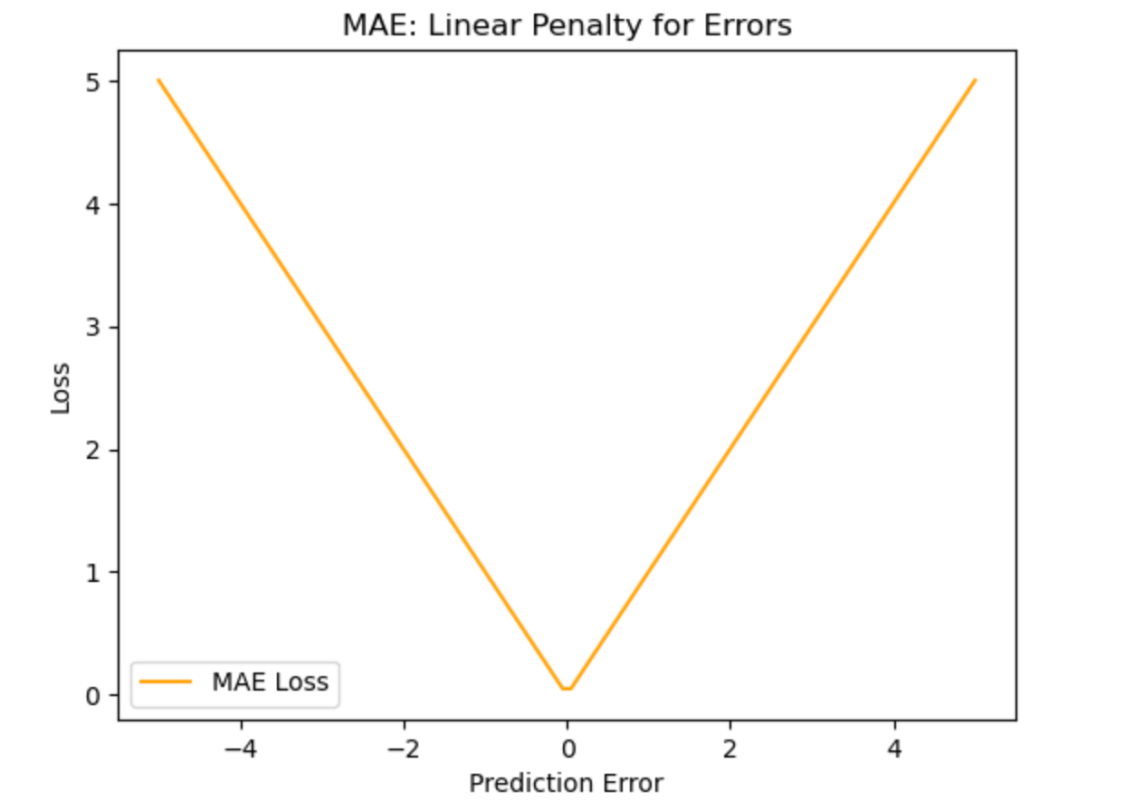
What the graph shows:
- The loss increases linearly with error.
- Outliers have proportional impact (unlike MSE's squared punishment).
C. Huber Loss (Smooth L1 Loss)
Huber loss combines the properties of both MSE and MAE. It behaves like MSE for smaller errors and like MAE for larger errors, making it less sensitive to outliers while still penalizing large mistakes.
Predicting the temperature for the next day. If the actual temperature is 30°C and the predicted temperature is 28°C, the model will be penalized for the error. However, if the prediction is 10°C off, Huber loss will reduce the impact of this large error compared to MSE.
Imagine: A coach who adjusts their feedback:
- For small mistakes (≤1 inch): "Focus on technique." (MSE-style)
- For big mistakes (>1 inch): "Just get closer next time." (MAE-style)
Where it's used:
- Self-driving cars (small steering errors corrected precisely, big errors handled safely)
- Stock trading (balance between precision and robustness)
Real Example:
In a self-driving car, small steering errors (1-2 degrees) are treated precisely, but huge errors (10+ degrees) are capped to prevent overreaction.
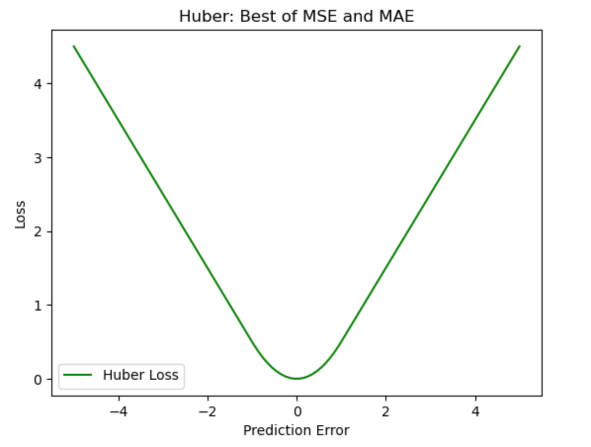
What the graph shows:
- Smooth curve near zero (like MSE for precision).
- Linear tails (like MAE for robustness).
2. Classification Loss Functions (For Categories)
A. Binary Cross-Entropy (Log Loss)
Measures performance for binary classification (Yes/No outcomes). It penalizes confident wrong predictions heavily.
Imagine: A teacher grading True/False tests:
- If you're 90% confident and right: "Good job!"
- If you're 90% confident and wrong: "FAIL! You should've doubted yourself!"
Where it's used:
- Spam filters (better to be unsure than confidently wrong)
- Cancer detection (false confidence is dangerous)
Real Example:
- Actual: Spam (1)
- Prediction 1: 0.9 (90% spam) → Loss = -log(0.9) ≈ 0.1
- Prediction 2: 0.1 (10% spam) → Loss = -log(0.1) ≈ 2.3 (harsh penalty!)
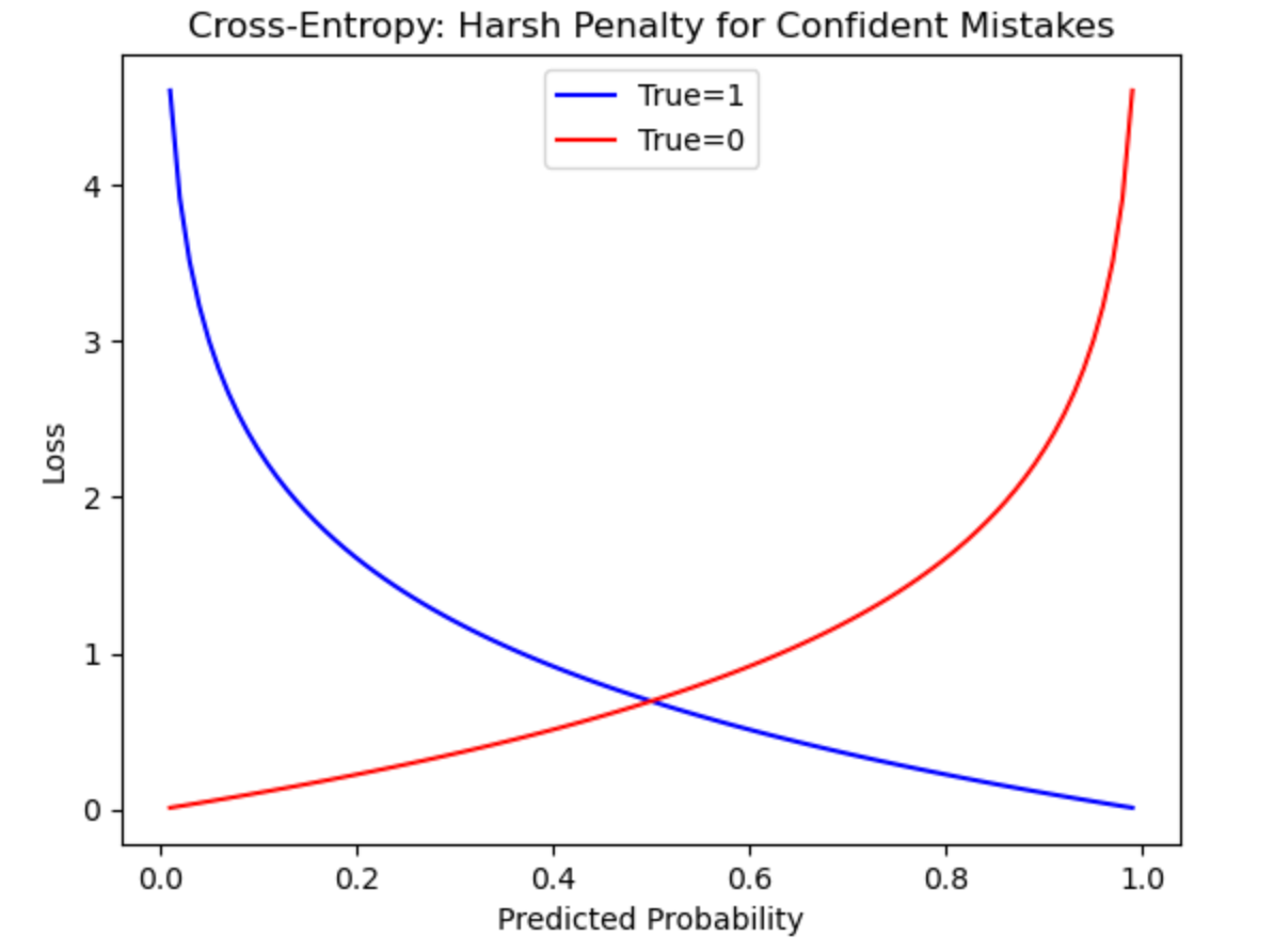
What the graph shows:
- Exponential rise when predictions are confidently wrong.
- Encourages the model to be certain only when correct
B. Categorical Cross-Entropy
Generalization of binary cross-entropy for multi-class problems (e.g., classifying cats, dogs, birds).
Imagine: Now the teacher grades multiple-choice exams:
- Only the correct answer's probability matters.
- Wrong answers? "I don’t care how wrong, just focus on the right one!"
Where it's used:
- Animal image classification (cat/dog/bird)
- News topic labeling (sports/politics/tech)
Real Example:
- True label: Cat
- Predictions: Cat (70%), Dog (20%), Bird (10%) → Loss = -log(0.70) ≈ 0.36
- If Cat was 30% → Loss = -log(0.30) ≈ 1.20 (much worse!)
Key Insight:
- The model only gets feedback on the correct class.
C. Hinge Loss (SVM Loss)
Hinge loss is a loss function primarily used for "maximum margin" classification, most notably in Support Vector Machines (SVMs).
Its key characteristic is that it doesn't just care about being right - it wants to be right by a safe margin.
Mathematical Definition
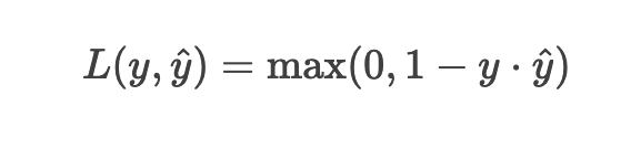
where:
- ( y ) = true label (-1 or +1 in SVMs)
- ( ŷ) = predicted score (not probability!)
How to Understand This? (With Examples)
1. Binary Classification Setup
Imagine we're classifying emails as spam (+1) or not spam (-1).
Our model outputs a raw score (not a probability):
- If score > 0 → predict "spam"
- If score < 0 → predict "not spam"
Hinge loss wants correct predictions to be not just barely correct, but correct by at least a margin of 1.
Case 1: Correct Classification with Good Margin
- True label (( y )): +1 (spam)
- Predicted score (( \hat{y} )): +2.5
- Calculation: ( \max(0, 1 - (1 \cdot 2.5)) = \max(0, -1.5) = 0 )
- Loss = 0 (because prediction is correct AND exceeds margin)
Case 2: Correct but Unsafe Classification
- True label: +1
- Predicted score: +0.8
- Calculation: ( \max(0, 1 - (1 \cdot 0.8)) = \max(0, 0.2) = 0.2 )
- Loss = 0.2 (correct but margin too small)
Case 3: Wrong Classification
- True label: +1
- Predicted score: -0.5
- Calculation: ( \max(0, 1 - (1 \cdot -0.5)) = \max(0, 1.5) = 1.5 )
- Loss = 1.5 (completely wrong prediction)
Visualizing Hinge Loss
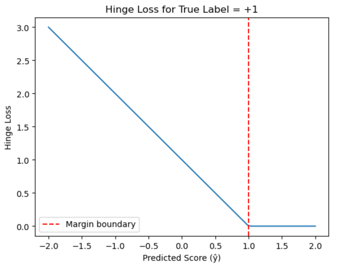
What the graph shows:
- Zero loss region (ŷ ≥ 1): Predictions are correct with sufficient margin
- Linear increase (ŷ < 1): Loss grows as predictions violate the margin
- The red dashed line marks the margin boundary
3. Advanced Loss Functions
A. Focal Loss (Handles Class Imbalance)
Focal Loss is a modified version of cross-entropy that helps the model focus more on difficult-to-classify examples by giving less importance to easy ones. It’s especially useful when working with imbalanced data, where some classes are rare.
Imagine you’re training a model to do something tough, like figuring out if a medical scan shows a rare disease. Most of the scans you’ve got are from healthy people—let’s say 95% healthy, 5% sick. If you use the standard error-checking method (cross-entropy), the model might just get lazy. It’ll focus on the 95% it can easily label as “healthy” and kinda shrug at the rare sick cases because they’re so few. It’s like a student cramming for the easy stuff and ignoring the hard questions—they still pass, but they miss the point.
Now, Focal Loss comes in like a smart coach. It says, “Hey, don’t waste so much energy on the easy stuff you already nailed. Let’s zoom in on the hard cases—the ones you keep messing up.” It does this by turning down the volume on the loss (the penalty) for examples the model’s already good at, and cranking it up for the tricky ones. So, in our disease example, it’s like telling the model, “Yeah, you’re great at spotting healthy scans, but let’s really grind on those rare disease cases until you get them right.”
Where it's used:
- Detecting tumors in X-rays (rare but critical)
- Fraud detection (most transactions are legit)
How it works:
- Reduces penalty for easy, common cases
- Focuses loss on hard, rare cases
Real Example:
- Without Focal Loss: Model ignores tumors (99% accuracy by guessing "healthy")
- With Focal Loss: Model forced to learn tumor patterns
B. Triplet Loss (Metric Learning)
Triplet Loss is used in metric learning tasks where the goal is to learn an embedding space where similar items are closer together and dissimilar items are farther apart.
Real-World Example: Face recognition. If the model is learning to recognize faces, triplet loss ensures that images of the same person are placed closer together in the embedding space, and images of different people are farther apart.
Imagine: A dance instructor teaching group coordination:
- Anchor: You
- Positive: Your dance partner (should move similarly)
- Negative: Random person (should move differently)
- Goal: Make sure you’re closer to your partner than to strangers.
Where it's used:
- Facial recognition (your face should be "close" to your other photos)
- Recommendation systems (similar users should get similar suggestions)
Real Example:
- Anchor: Your profile photo
- Positive: Another photo of you with glasses
- Negative: A photo of your friend
- Loss: Ensures your two photos are more alike than yours and your friend’s
C. Custom Loss - The Problem-Specific Tool
Custom loss functions are tailored to specific tasks where standard loss functions may not work well. They are designed to meet the unique needs of the problem.
Real-World Example: In a recommendation system, a custom loss function might be created to optimize not just prediction accuracy, but also the diversity of recommendations, ensuring the model recommends a wide variety of items rather than similar ones.
Imagine: A chef judging a dish:
- Normal rule: "Taste = 70%, Presentation = 30%"
- Custom rule: "For hospital meals, Nutrition = 50%, Taste = 30%, Allergens = 20%"
Where it's used:
- Medical AI (higher penalty for missing diseases)
- Self-driving cars (harsher penalty for false "safe" predictions)
This is cool, two AIs, talking about loss function and discussing the types and examples: [Must listen]
Choosing Your Loss Function
| Problem Type | Recommended Loss | Why? |
|---|---|---|
| Predicting prices | MSE, Huber | Precision + robustness |
| Medical diagnosis | MAE, Custom | Avoid catastrophic misses |
| Spam detection | Cross-Entropy | Confidence matters |
| Rare events (e.g., fraud) | Focal Loss | Focuses on the important few |
| Face recognition | Triplet Loss | Learns similarity, not just labels |