Core Machine Learning Concepts Part 2 - Optimization
Explore optimization in machine learning! See how algorithms adjust parameters to minimize loss, guiding models to better predictions step by step.
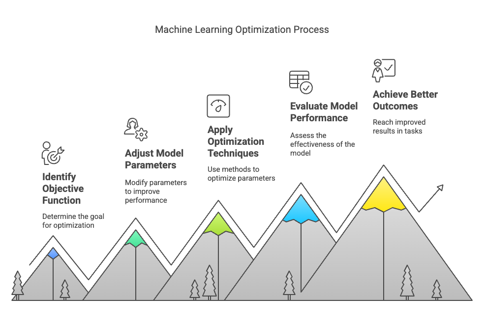
Optimization is a critical concept in machine learning (ML) and artificial intelligence (AI). It helps improve the performance of models by adjusting parameters in the right direction. This process ensures that the model learns from the data efficiently and makes accurate predictions.
Optimization is how machines learn from mistakes.
Imagine teaching a child to catch a ball:
- The child tries (initial prediction)
- Sees how far they missed (calculates loss)
- Adjusts their position (updates model parameters)
- Repeats until they catch perfectly (minimizes error)
In technical terms:
- Objective: Find model parameters (weights) that minimize a loss function
- Process: Iteratively adjust weights to reduce prediction errors
- Analogy: Like tuning a radio dial to get the clearest signal
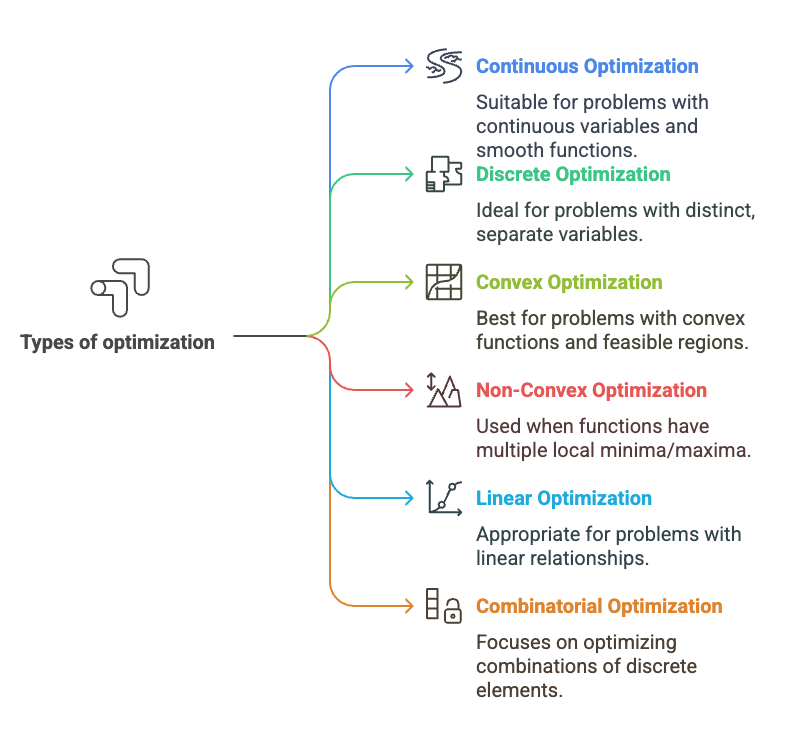
It’s about finding the best solution to a problem when you’ve got some choices and a goal. In machine learning (and beyond), that goal is usually minimizing something (like errors) or maximizing something (like accuracy).
When we train a machine learning model, we need to adjust its parameters (like weights in a neural network) so that the model's predictions are as accurate as possible. This process is what optimization helps us with.
Think of it like tuning a guitar. You twist the pegs until the strings sound just right. Optimization is the process of tweaking until you hit that sweet spot.
Key Pieces
- Goal (Objective Function): This is what you’re trying to improve, like minimizing “loss” (how wrong your model is) or maximizing “profit.”
- Choices (Parameters): These are the knobs you can turn—like the weights in a neural network or the route you pick for your trip.
- Limits (Constraints): Sometimes you’ve got rules—like a budget or a deadline—that box you in.
Popular Optimization Algorithms
- Gradient Descent (GD)
- Stochastic Gradient Descent (SGD)
- Mini-Batch Gradient Descent
- Momentum
- Adam (Adaptive Moment Estimation)
- RMSprop
- Adagrad
- L-BFGS
- Lion (2023)
- Sophia (2023)
1. Gradient Descent
Gradient Descent is a popular optimization technique that adjusts the parameters of a model by moving in the direction of the steepest decrease in the loss function. It iterates over the data, calculating the gradient (the derivative) of the loss function with respect to the model parameters, and then updates the parameters accordingly. The goal is to reach the minimum value of the loss function.
Gradient descent is the most commonly used optimization algorithm in machine learning, especially for deep learning.
How it works:
- Imagine you are at the top of a hill (the loss function is high here) and want to reach the bottom (where the loss is minimized).
- The gradient is the slope of the hill, which tells you in which direction to move.
- Gradient descent calculates the gradient and adjusts the model parameters in the direction of the steepest decrease in the loss.
If you're training a neural network and want to minimize the error in your predictions, gradient descent will update the weights of the network to make the predictions more accurate.
Let's visualise this:
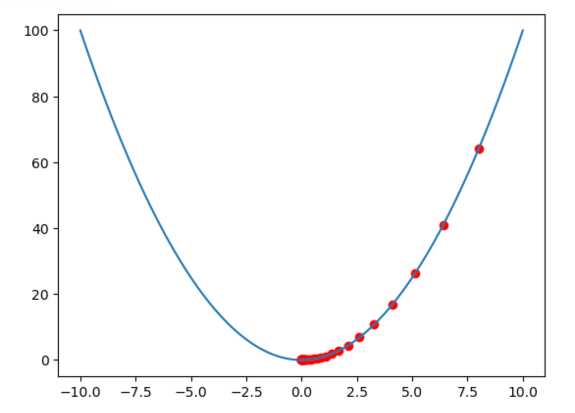
What does This Visualization Show?
This graph demonstrates gradient descent optimization using a simple parabola (y = x²) as our loss function. Imagine this parabola as a valley that an AI "hiker" is trying to descend to find the lowest point (minimum loss).
Key Components
- The Valley (Blue Curve)
- Shape: Parabola (
y = x²) - Minimum:
x=0, y=0(optimal model performance)
- Shape: Parabola (
- The Hiker (Red Dots)
- Starts at
x=8(high loss:64) - Moves downhill using gradient descent
- Starts at
- The Algorithm's Steps
- Slope Calculation:
2 × current x-position
- Slope Calculation:
Update Rule:
new_x = current_x - (0.1 × slope)
Step-by-Step Movement (First 5 Steps)
| Step | Position (x) | Slope (2×x) |
Update (x - 0.1×slope) |
New x | Loss (x²) |
|---|---|---|---|---|---|
| 1 | 8.0 | 16.0 | 8.0 - (0.1×16) = 6.4 | 6.4 | 40.96 |
| 2 | 6.4 | 12.8 | 6.4 - (0.1×12.8) = 5.12 | 5.12 | 26.21 |
| 3 | 5.12 | 10.24 | 5.12 - (0.1×10.24) = 4.096 | 4.096 | 16.78 |
| 4 | 4.096 | 8.192 | 4.096 - (0.1×8.192) = 3.277 | 3.277 | 10.74 |
| 5 | 3.277 | 6.554 | 3.277 - (0.1×6.554) = 2.622 | 2.622 | 6.87 |
Smaller steps (lr=0.1) means more steps to reach the minimum.
lr is the Learning rate:
The learning rate is a hyperparameter that controls how much the model's parameters are adjusted with each step during training. A higher learning rate means bigger updates, while a lower rate results in smaller, more gradual adjustments.
Loss decreases steadily:64 → 40.96 → 26.21 → ... → near 0.
Why This Matters
- Goldilocks Principle:
lr=0.9→ Too large (overshoots)lr=0.1→ Just right (smooth convergence)lr=0.01→ Too small (extremely slow)
Try This!
Change lr to see how it affects the hiker’s path:
lr=0.1: Slow but steady convergence.lr=1.5: Wild oscillations (fails to converge).
This shows how critical the learning rate is in training AI models. 🚀
Code:
import matplotlib.pyplot as plt
import numpy as np

# Create a valley (loss function)
x = np.linspace(-10, 10, 100)
y = x**2  # Simple parabola representing the loss function

# Hiker's journey
positions = [8]  # Start at x=8
lr = 0.1  # Learning rate

# Perform gradient descent
for _ in range(50):  # 20 iterations for gradient descent
    slope = 2 * positions[-1]  # Derivative of x^2 is 2x
    positions.append(positions[-1] - lr * slope)  # Update position using gradient

# Plot the loss function and hiker's journey
plt.plot(x, y)  # Plot the loss function (x^2)
plt.scatter(positions, [p**2 for p in positions], c='red')  # Plot hiker's journey (red points)
plt.show()  # Display the plot
2. Stochastic Gradient Descent (SGD)
SGD is a variation of gradient descent. Instead of computing the gradient using the entire dataset (which can be slow), it uses only one data point (or a small batch) to update the parameters.
How it works:
- By using smaller chunks of data, the updates happen more frequently, which makes the optimization process faster.
- The downside is that the path towards the minimum can be "noisy," but with enough iterations, it will still converge.
Example: Imagine you're trying to solve a math problem using gradient descent. Instead of looking at all the problems, SGD looks at just one at a time. Although it's faster, the solution may oscillate a bit before finding the best one.
3. Mini-batch Gradient Descent
Mini-batch gradient descent is a combination of both batch and stochastic gradient descent. It updates the parameters using a small subset (batch) of data rather than the whole dataset or just one data point.
How it works:
- It’s faster than standard gradient descent because it uses less data at a time but still benefits from more stable updates compared to SGD.
Example: In training deep learning models, mini-batch gradient descent is often used to balance speed and accuracy. A batch might include 32, 64, or 128 data points.
Real-Life Examples:
- Netflix Recommendations
- Optimization: Adjusts weights to minimize your "dislike" clicks
- Algorithm: Adam optimizer
- Impact: Better suggestions = longer viewing
- Self-Driving Cars
- Optimization: Tweaks neural network weights to minimize steering errors
- Algorithm: SGD with Momentum
- Impact: Smoother turns, safer rides
"Optimizers are the unsung heroes of AI - while architectures get glory, optimizers do the hard work of learning." - Yann LeCun