Core Machine Learning Concepts Part 3 - Gradient Descent
Curious about how AI models improve their predictions over time? In just 10 minutes, we’ll break down how Gradient Descent helps models reduce errors and get smarter with every step—without the need for complex math!
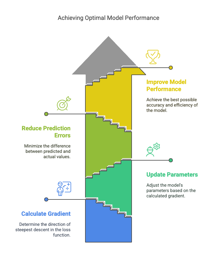
Gradient Descent is a key method used in machine learning and Neural Networks to improve predictions by reducing errors. It works by adjusting the model's settings—such as weights and biases—based on how far off the predictions are from the actual values.
Imagine an AI model trained to predict whether an image is of a dog or a cat. When an image is fed to the model, if it makes an error, the model calculates the loss (how far off the prediction is). Gradient Descent then adjusts the model’s weights and biases to reduce this error. Through backpropagation, these adjustments are made across the network, and the model is updated. This process continues with each new image, gradually minimizing the loss and improving the model's accuracy over time.
Our mission: Minimize the loss function (reducing the gap between predicted and actual values) to achieve maximum model accuracy.
Let's try to imagine this.
Imagine standing on top of a hill (the error surface) and wanting to reach the lowest point (the minimum error). Gradient Descent helps by calculating the slope (gradient) of the hill at your current position and telling you which direction to move. It updates your position toward the steepest descent, reducing the error step by step. This process repeats until the model reaches the best predictions possible. The smaller the error (loss), the better the model's predictions. It's like a hiker trying to find the lowest point in a valley by taking small, calculated steps downhill based on the difference between the model's predictions and the true values.
The size of each step is controlled by the learning rate, which determines how quickly or slowly the model adjusts. The goal is to minimize the error or "cost" to make the model as accurate as possible.
Reaching the lowest point of the error function isn’t something that happens all at once. AI models are complex, and sometimes they get stuck in a "local minima," which is like a small dip in the landscape that seems like the lowest point, but it’s not the best overall. The true goal is to reach the "global minima," which is the absolute lowest point across the entire landscape.
Think of it like trying to find the lowest point in a big mountain range—sometimes, you might find a small valley that looks like the lowest, but the global minima is the deepest valley overall. Only when the model reaches this point can we say it has the least error and is performing at its best.
Model 'learning rate' is crucial for guiding the model to the lowest point of the loss function.
- With a low learning rate, the model behaves like a wise man, the model makes very small adjustments to its weights and biases to minimize the loss function. While this prevents the model from overshooting the optimal solution, it can cause the model to move too slowly and may get stuck in local minima (suboptimal points) without exploring other, potentially better solutions. The model might also take a very long time to converge to the global minimum, which can make the training process inefficient and slow. Essentially, the model moves cautiously but might not make significant progress if the learning rate is too small.
- A higher learning rate can cause a zig-zag movement because the model makes large, erratic adjustments to its weights and biases in an attempt to minimize the error. When the learning rate is too high, the steps taken by the model are too large. This causes the model to overshoot the global minimum and jump over the optimal solution. It then corrects itself in the opposite direction, resulting in a zig-zag pattern. This unstable movement prevents the model from smoothly converging to the optimal solution, making the learning process inefficient and inaccurate.
Choosing the optimal learning rate is crucial for efficient model training. One approach is using learning rate schedules, starting high and gradually lowering it to refine the model's adjustments. Another method is the learning rate finder, where you gradually increase the rate and track the point of fastest loss reduction. Techniques like grid or random search test different rates for the best performance. Algorithms like Adam adjust the learning rate automatically based on gradients. Monitoring validation loss during training helps identify if the learning rate is appropriate—smooth loss suggests a good rate, while fluctuating or increasing loss signals a need for adjustment.
Let's play around with it. You can change the value of lr and see how the model reaches the lowest point of the error function:
The Code:
import matplotlib.pyplot as plt
import numpy as np
# Create the valley (loss function)
x = np.linspace(-10, 10, 100)
y = x**2 # Simple parabola representing the loss function
# Define the starting points (representing different loss scenarios)
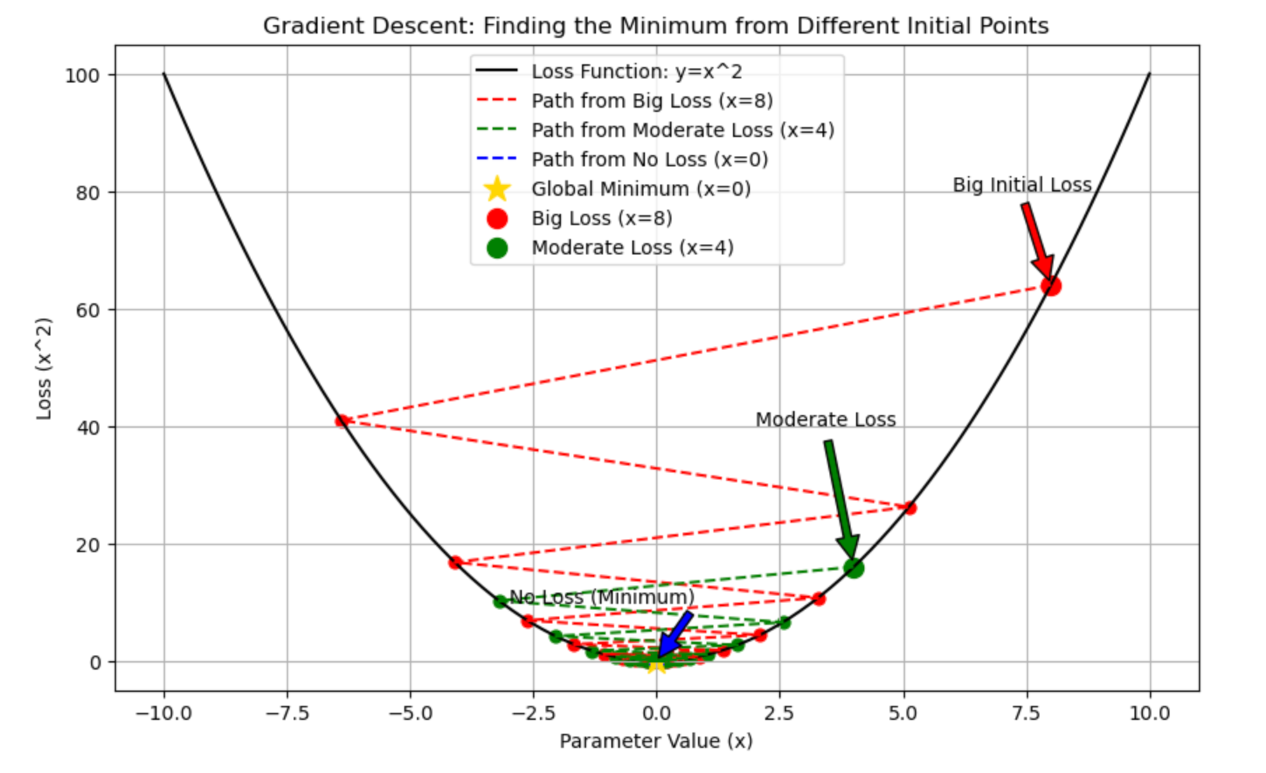
starting_positions = [8, 4, 0] # Big Loss, Moderate Loss, No Loss
labels = ['Big Loss (x=8)', 'Moderate Loss (x=4)', 'No Loss (x=0)']
colors = ['red', 'green', 'blue']
# Learning rate for gradient descent
lr = 0.9
# Set up the figure and plot the loss function
fig, ax = plt.subplots(figsize=(10, 6))
ax.plot(x, y, label="Loss Function: y=x^2", color='black')
# Hiker's journey from different starting points
for start, label, color in zip(starting_positions, labels, colors):
positions = [start]
for _ in range(20): # 20 iterations for gradient descent
slope = 2 * positions[-1] # Derivative of x^2 is 2x
new_pos = positions[-1] - lr * slope
positions.append(new_pos)
# Plot the path taken by the optimizer
ax.plot(positions, [p**2 for p in positions], color=color, linestyle='--', label=f"Path from {label}")
ax.scatter(positions, [p**2 for p in positions], c=color, s=40)
# Add special markers for the minimum and the starting points
ax.scatter([0], [0], c='gold', s=200, marker='*', label="Global Minimum (x=0)")
ax.scatter([8], [64], c='red', s=100, marker='o', label="Big Loss (x=8)")
ax.scatter([4], [16], c='green', s=100, marker='o', label="Moderate Loss (x=4)")
# Annotate the starting points and the minimum
ax.annotate('Big Initial Loss', xy=(8, 64), xytext=(6, 80),
arrowprops=dict(facecolor='red', shrink=0.05))
ax.annotate('Moderate Loss', xy=(4, 16), xytext=(2, 40),
arrowprops=dict(facecolor='green', shrink=0.05))
ax.annotate('No Loss (Minimum)', xy=(0, 0), xytext=(-3, 10),
arrowprops=dict(facecolor='blue', shrink=0.05))
# Set plot labels and title
ax.set_xlabel('Parameter Value (x)')
ax.set_ylabel('Loss (x^2)')
ax.set_title('Gradient Descent: Finding the Minimum from Different Initial Points')
ax.legend()
ax.grid(True)
# Show the plot
plt.show()Result with lr = .9
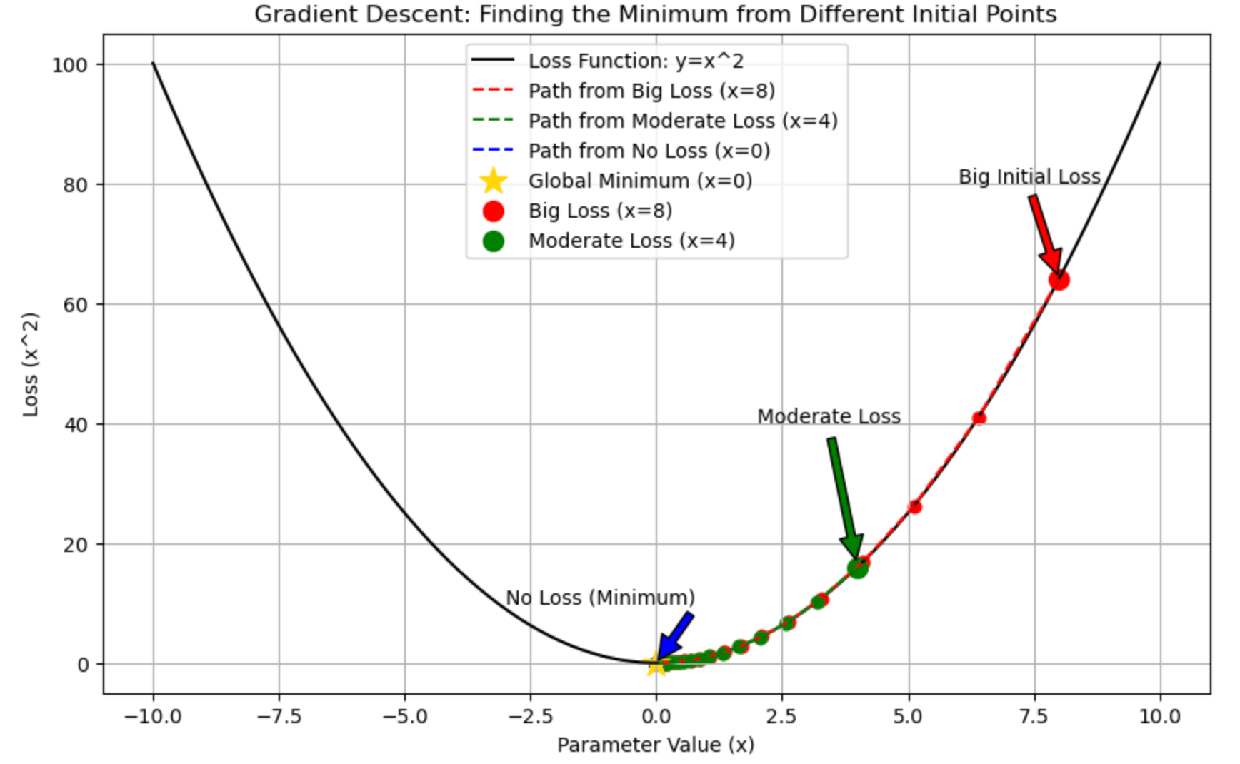
Result with lr = .1
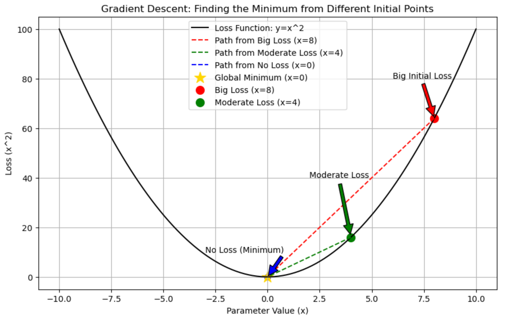
Result with lr = .5
Let's see the iterations for model improvisation.
Example 1:
In this example, we create a simple dataset where y depends on x in a linear way, but with some random noise added. Our goal is to use Gradient Descent to find the best weight (w) and bias (b) for the model so that it can predict y from x as accurately as possible.
- Dataset: We generate 100 random numbers for
xbetween 0 and 10, andyis calculated as a linear equation (y = 2.5 * x + some noise). - Goal: We start with random values for
wandb, then use Gradient Descent to adjust these values so the model can make better predictions by minimizing the error.
The Code:
import numpy as np
import matplotlib.pyplot as plt
# Generate a simple dataset
np.random.seed(42)
x = np.random.rand(100, 1) * 10 # Random data points between 0 and 10
y = 2.5 * x + np.random.randn(100, 1) * 2 # Linear relationship with some noise
# Initialize weights and bias
w = np.random.randn(1) # Random initial weight
b = np.random.randn(1) # Random initial bias
# Hyperparameters
learning_rate = 0.01
iterations = 100
m = len(x)
# Store gradients for plotting
gradients = []
# Gradient Descent
for i in range(iterations):
# Predictions
y_pred = w * x + b
# Calculate the loss (Mean Squared Error)
loss = np.mean((y_pred - y) ** 2)
# Compute gradients (derivatives of the loss function w.r.t. w and b)
dw = (2/m) * np.sum((y_pred - y) * x)
db = (2/m) * np.sum(y_pred - y)
# Store gradients for visualization
gradients.append((dw, db))
# Update weights and bias
w -= learning_rate * dw
b -= learning_rate * db
# Print loss every 10 iterations for monitoring
if i % 10 == 0:
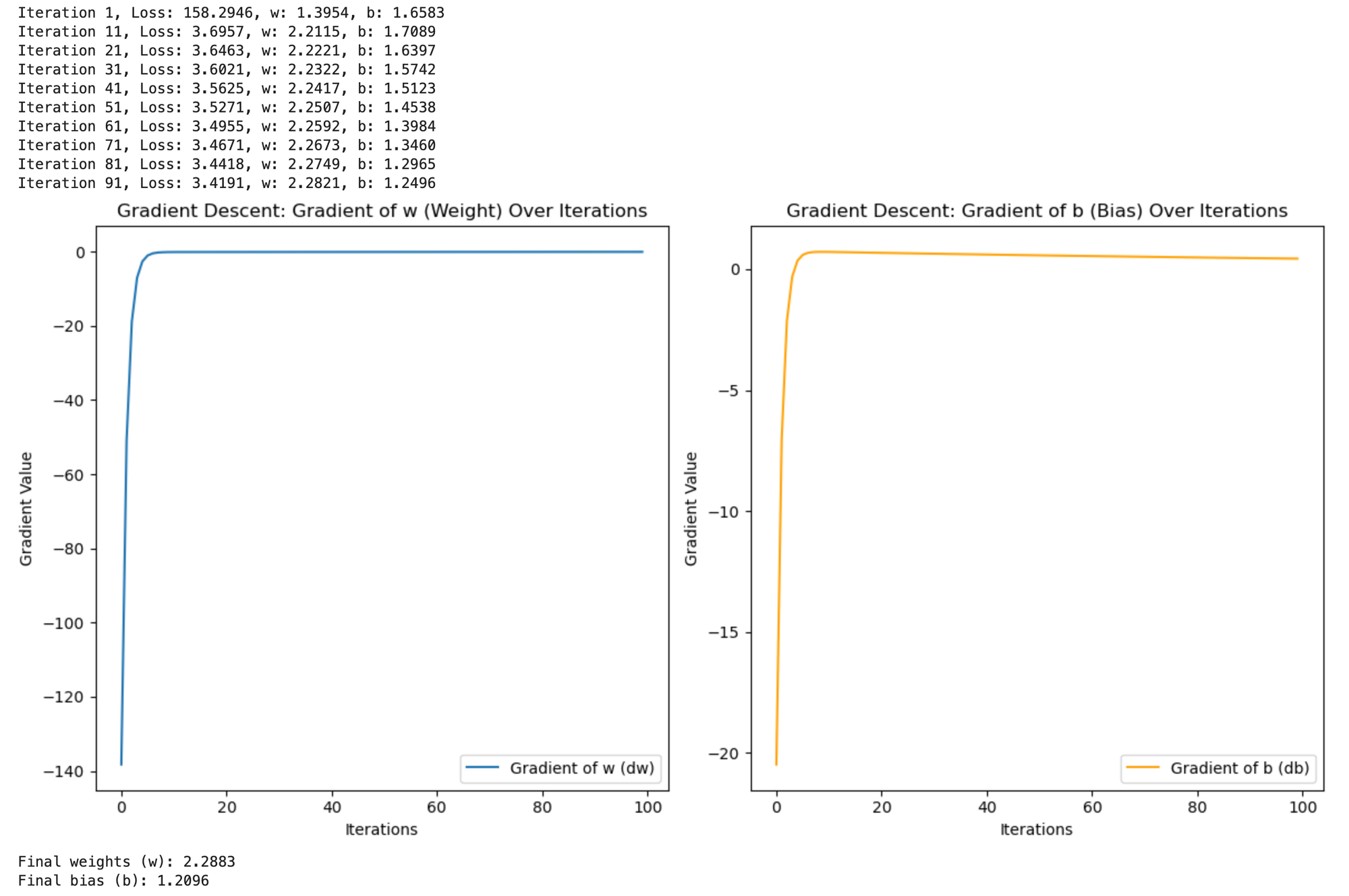
print(f"Iteration {i+1}, Loss: {loss:.4f}, w: {w[0]:.4f}, b: {b[0]:.4f}")
# Extract gradients for plotting
dw_values, db_values = zip(*gradients)
# Plotting the gradient values
plt.figure(figsize=(12, 6))
# Plot gradient for w (weight)
plt.subplot(1, 2, 1)
plt.plot(dw_values, label="Gradient of w (dw)")
plt.xlabel("Iterations")
plt.ylabel("Gradient Value")
plt.title("Gradient Descent: Gradient of w (Weight) Over Iterations")
plt.legend()
# Plot gradient for b (bias)
plt.subplot(1, 2, 2)
plt.plot(db_values, label="Gradient of b (db)", color='orange')
plt.xlabel("Iterations")
plt.ylabel("Gradient Value")
plt.title("Gradient Descent: Gradient of b (Bias) Over Iterations")
plt.legend()
plt.tight_layout()
plt.show()
# Final results
print(f"Final weights (w): {w[0]:.4f}")
print(f"Final bias (b): {b[0]:.4f}")Result:
How It Worked-
The Gradient Descent algorithm works by gradually adjusting the model's parameters (weight w and bias b) to reduce the difference between predicted values (y_pred) and the actual values (y). Here's how it works:
- Gradients: In each step, the algorithm calculates how much the weight and bias need to change to reduce the error. This is called the "gradient."
- Updates: The model then updates the weight and bias in the right direction (based on the gradient) to make its predictions more accurate.
- Learning: At first, the changes to the weight and bias are large. But as the model gets better, the changes become smaller because it is getting closer to the best solution.
- Final Result: After running for several steps, the model finds the best weight and bias that minimize the error, allowing it to predict
ymore accurately. The graphs show how the gradients decrease over time, showing how the model learns.
Example 2:
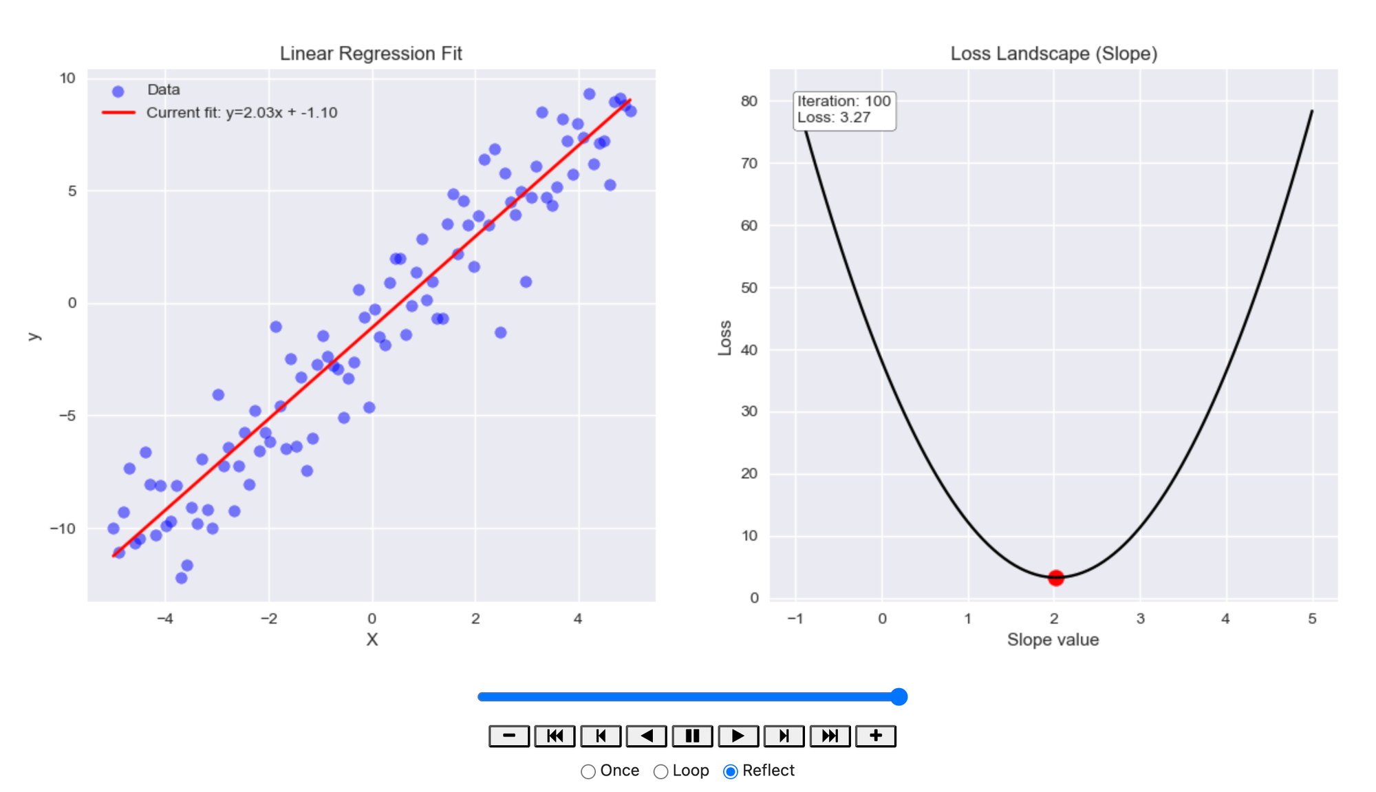
In this example, we are using Gradient Descent to fit a linear regression model to some synthetic data. The goal is to adjust the slope and intercept of the line that best fits the data points. We simulate this process by randomly generating data points that follow a linear relationship with some noise added.
- Dataset: We create
xvalues between -5 and 5, and generate the correspondingyvalues using a linear equation (y = 2.5 * x - 1) with some random noise added. - Model: The model starts with random initial values for slope (
w) and intercept (b) and uses Gradient Descent to adjust these values in order to minimize the error (loss) between the predicted and actualyvalues. - Goal: Use Gradient Descent to find the optimal slope and intercept that best fit the data.
The Code:
import numpy as np
import matplotlib.pyplot as plt
from matplotlib.animation import FuncAnimation
from IPython.display import HTML

# Set up the figure and axis
plt.style.use('seaborn-v0_8')  # Updated style name for newer matplotlib versions
fig, (ax1, ax2) = plt.subplots(1, 2, figsize=(14, 6))

# Generate synthetic data
np.random.seed(42)
X = np.linspace(-5, 5, 100)
true_slope = 2
true_intercept = -1
y = true_slope * X + true_intercept + np.random.normal(0, 2, 100)

# Initialize parameters (weights and bias)
slope = np.random.randn()
intercept = np.random.randn()
learning_rate = 0.01
iterations = 100

# Store history for visualization
slope_history = []
intercept_history = []
loss_history = []

# Gradient Descent
for i in range(iterations):
    # Predictions
    y_pred = slope * X + intercept

    # Calculate loss (Mean Squared Error)
    loss = np.mean((y_pred - y)**2)

    # Calculate gradients
    grad_slope = 2 * np.mean((y_pred - y) * X)
    grad_intercept = 2 * np.mean(y_pred - y)

    # Update parameters
    slope = slope - learning_rate * grad_slope
    intercept = intercept - learning_rate * grad_intercept

    # Store history
    slope_history.append(slope)
    intercept_history.append(intercept)
    loss_history.append(loss)

# Function to update animation frames
def update(frame):
    ax1.clear()
    ax2.clear()

    current_slope = slope_history[frame]
    current_intercept = intercept_history[frame]
    current_loss = loss_history[frame]

    # Plot data and current fit
    ax1.scatter(X, y, color='blue', alpha=0.5, label='Data')
    current_line = current_slope * X + current_intercept
    ax1.plot(X, current_line, color='red', linewidth=2,
             label=f'Current fit: y={current_slope:.2f}x + {current_intercept:.2f}')
    ax1.set_title('Linear Regression Fit')
    ax1.set_xlabel('X')
    ax1.set_ylabel('y')
    ax1.legend()

    # Plot loss landscape (simplified 2D view)
    s = np.linspace(true_slope-3, true_slope+3, 100)
    losses = [np.mean(((s_i * X + current_intercept) - y)**2) for s_i in s]
    ax2.plot(s, losses, color='black')
    ax2.scatter([current_slope], [current_loss], color='red', s=100)

    # Add gradient arrow
    arrow_length = 0.5  # Scale for visualization
    if frame < len(slope_history)-1:
        next_slope = slope_history[frame+1]
        next_loss = np.mean(((next_slope * X + current_intercept) - y)**2)
        ax2.arrow(current_slope, current_loss,
                 (next_slope - current_slope)*arrow_length,
                 (next_loss - current_loss)*arrow_length,
                 head_width=0.1, head_length=0.1, fc='red', ec='red')

    ax2.set_title('Loss Landscape (Slope)')
    ax2.set_xlabel('Slope value')
    ax2.set_ylabel('Loss')
    ax2.annotate(f'Iteration: {frame+1}\nLoss: {current_loss:.2f}',
                xy=(0.05, 0.9), xycoords='axes fraction',
                bbox=dict(boxstyle="round", fc="white"))

    # Draw angle indicator
    if frame > 0 and frame < len(slope_history)-1:
        prev_slope = slope_history[frame-1]
        prev_loss = np.mean(((prev_slope * X + current_intercept) - y)**2)

        # Calculate angle (in degrees)
        dx1 = current_slope - prev_slope
        dy1 = current_loss - prev_loss
        dx2 = next_slope - current_slope
        dy2 = next_loss - current_loss

        angle = np.degrees(np.arctan2(dy2, dx2) - np.arctan2(dy1, dx1))
        if angle < 0:
            angle += 360

        ax2.annotate(f'Angle: {angle:.1f}°',
                    xy=(current_slope, current_loss),
                    xytext=(10, 20), textcoords='offset points',
                    arrowprops=dict(arrowstyle="->"))

# Create animation
ani = FuncAnimation(fig, update, frames=iterations, interval=200, repeat=False)
plt.close()

# Display animation
HTML(ani.to_jshtml())Result:
How It Worked:
The code implements Gradient Descent by iteratively updating the slope and intercept to reduce the error between the predicted and actual y values:
- Gradients Calculation: In each iteration, the algorithm calculates how much the slope and intercept need to be adjusted to reduce the loss. This is done by computing the gradients for both the slope (
dw) and the intercept (db). - Model Updates: Using the gradients, the model adjusts the slope and intercept by a small amount determined by the learning rate.
- Visualization: The animation shows two things:
- Linear Regression Fit: The scatter plot of data points and the red line representing the model's current fit. As the model learns, the line gets closer to the optimal fit.
- Loss Landscape: A graph showing how the loss changes with different slope values. The red dot shows the current loss, and an arrow indicates the direction of the next update. Additionally, an angle indicator visualizes the direction change between iterations, showing the model’s path as it converges to the optimal solution.
As the animation progresses:
- The slope and intercept values are updated to minimize the error.
- The loss decreases over time, and the model’s fit becomes more accurate.
- The loss landscape graph visualizes how the gradient guides the model toward the minimum loss.
The animation shows how the model gradually converges to the optimal solution, with the line fitting the data better and the loss decreasing to its lowest value. The gradient arrows and angle indicator help visualize how the slope is adjusted step by step.
Types of Gradient Descent
- Batch Gradient Descent:
- Stochastic Gradient Descent
- Mini-batch Gradient Descent
- Batch Gradient Descent:
- This type sums the entries for each point in a training set.
- It updates the model only after all the training examples have been evaluated. This is why it's called "batch".
- In terms of computational efficiency, it is described as computationally effective, getting a high rating.
- However, it can result in long processing times when using large training data sets.
- It also needs to store all of that data in memory to process it.
- Stochastic Gradient Descent:
- This method evaluates each training example, but one at a time.
- Since it only needs to hold one training example at a time, the examples are easy to store in memory.
- It can get individual responses much faster.
- In terms of speed, it is described as fast.
- However, its computational efficiency is described as lower.
- Mini-batch Gradient Descent:
- This is described as a "happy medium" between Batch and Stochastic Gradient Descent.
- It splits the training data set into small batch sizes.
- It performs updates on each of those smaller batches.
- This approach offers a nice balance of computational efficiency and speed.
| Feature | Batch Gradient Descent (BGD) | Stochastic Gradient Descent (SGD) | Mini-batch Gradient Descent (MBGD) |
|---|---|---|---|
| Definition | Uses the entire dataset to compute gradients for each update. | Uses a single training example to compute the gradient for each update. | Uses a small subset (mini-batch) of the dataset for each update. |
| Convergence Speed | Slow for large datasets, but stable. | Fast, updates are frequent but noisy. | Balanced, faster than BGD and less noisy than SGD. |
| Computation Cost | High, as it needs to process the entire dataset. | Low, since it only processes one data point at a time. | Moderate, processes smaller subsets of data in each update. |
| Memory Requirements | High, as it needs to store the entire dataset. | Low, as only one data point is processed at a time. | Moderate, stores only the mini-batch in memory. |
| Noise in Updates | No noise, very stable. | High noise due to single data points being used. | Lower noise, as mini-batches help smooth updates. |
| Accuracy | Tends to converge to a global minimum, but slowly. | May oscillate around the minimum due to high variance. | Generally provides a good balance between speed and accuracy. |
| Suitability | Suitable for small datasets where computational cost is not an issue. | Suitable for large datasets with noisy data. | Suitable for large datasets, balancing speed and accuracy. |
| Update Frequency | One update per full pass through the dataset (epoch). | One update per data point. | One update per mini-batch. |
| Example Use Case | Small-scale datasets, where stability is important. | Large datasets, or online learning (real-time updates). | Large datasets, balancing speed and convergence. |