[Day 13] Supervised Machine Learning Type 4 - Support Vector Machine (with a Small Python Project)
How do machines draw the perfect line between “yes” & “no”? Discover the magic of SVM with real examples and a flower-predicting Python project!
![[Day 13] Supervised Machine Learning Type 4 - Support Vector Machine (with a Small Python Project)](https://storage.ghost.io/c/55/e8/55e827ca-bf8d-4eee-bdb4-ee48e49a011a/content/images/size/w2000/2025/03/_--visual-selection--13-.svg)
Understanding Support Vector Machine (SVM) for Binary Classification
Support Vector Machine (SVM) is a supervised learning algorithm that excels at solving classification problems. Its primary goal is to separate data points into two distinct categories by finding the best-dividing boundary, called the hyperplane. SVM is particularly effective when working with high-dimensional data or when the classes are not easily separable in their original space.
Key Concepts Simplified
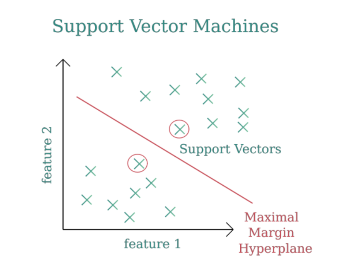
1. Hyperplane
The hyperplane is the dividing line (or surface in higher dimensions) that separates data points of different classes. Think of it as the "decision boundary" that determines which class a new data point belongs to. For example:
- If you’re classifying emails as spam or not spam, the hyperplane is the rule that divides these two categories.
- In 2D, it’s a straight line; in 3D, it’s a flat surface.
2. Support Vectors
Support vectors are the most influential data points in the dataset. These are the points closest to the hyperplane and essentially define its position.
- Imagine a fence being held by poles—these poles are your support vectors. Moving them changes the position of the fence (hyperplane).
- For SVM, only these crucial points matter, making it robust against irrelevant data points or outliers.
3. Margin
The margin is the distance between the hyperplane and the nearest data points (support vectors).
- Goal of SVM: Maximize this margin. A larger margin means a more confident and generalizable decision boundary.
- Think of it as ensuring there's enough "buffer space" on either side of the dividing line to handle unseen data better.
You can understand it better with this article:
Understand the concept in the below video:
How Does Support Vector Machine Work?
- Linear SVM: In the case of linearly separable data, SVM tries to find the line (or hyperplane) that best separates the two classes while maximizing the margin between the classes.
- Non-linear SVM: If the data is not linearly separable, SVM uses a kernel trick to transform the data into a higher-dimensional space where a linear separation is possible. Common kernels include polynomial and RBF (Radial Basis Function) kernels.
Advantages of Support Vector Machine:
- Effective in High Dimensional Spaces: SVM is effective when the number of features is larger than the number of samples.
- Robust to Overfitting: SVM is less prone to overfitting, especially in high-dimensional spaces, as it tries to find the maximum margin that generalizes well.
- Works Well with Non-linear Data: By using kernels, SVM can handle non-linearly separable data, making it versatile for various datasets.
Limitations of Support Vector Machine:
- Computationally Intensive: SVM can be computationally expensive, especially when the dataset is large or has a large number of features.
- Memory Usage: SVM can be memory-intensive due to the requirement of storing large amounts of data (especially with non-linear kernels).
- Parameter Tuning: SVM requires careful tuning of parameters such as the regularization parameter and the choice of kernel, which can be time-consuming.
Real-Life Use Cases for Support Vector Machine (SVM):
Here are five real-life applications where Support Vector Machine can be used effectively:
1. Medical Diagnosis (Cancer Detection)
- Problem: Classifying whether a tumor is malignant or benign based on medical features.
- Example: The Breast Cancer dataset contains features such as tumor size, shape, and texture, and SVM can classify whether the tumor is malignant or benign.
- Why SVM: SVM is well-suited for medical classification problems where the features are high-dimensional, and the data is complex and non-linear.
2. Image Classification
- Problem: Classifying images into different categories (e.g., cat vs. dog, handwritten digits).
- Example: In image recognition, SVM can classify objects based on pixel values and feature extraction techniques (such as Histogram of Oriented Gradients - HOG).
- Why SVM: SVM handles high-dimensional image data efficiently, especially when combined with feature extraction techniques.
3. Text Classification (Spam vs. Non-Spam Email)
- Problem: Classifying emails as either spam or non-spam based on content.
- Example: An email provider can use SVM to classify incoming emails as spam or not based on the frequency of certain words, sender information, etc.
- Why SVM: SVM is particularly useful for text classification, where the data has high dimensionality due to the large vocabulary of words.
4. Financial Market Predictions (Credit Scoring)
- Problem: Predicting whether a customer is likely to default on a loan based on their financial history and attributes.
- Example: Banks can use SVM to classify customers as high-risk or low-risk based on features like credit score, income, and loan history.
- Why SVM: Financial data often involves complex relationships and can benefit from the non-linear capabilities of SVM to classify risk levels.
5. Bioinformatics (Protein Classification)
- Problem: Classifying proteins based on their structure and function.
- Example: In bioinformatics, SVM is used to predict whether a protein sequence belongs to a specific class, such as predicting whether a protein sequence is part of a family of enzymes or not.
- Why SVM: SVM handles high-dimensional biological data and can be used with various kernels to address non-linear relationships.
Quick Python Project:
In this project, we are tasked with classifying flowers into 6 species (e.g., Rose, Tulip, Daisy, Orchid, Lily, and Sunflower) based on 10 input features. The features include measurements such as leaf length, petal length, stem height, etc., and the goal is to predict which species the flower belongs to.
Dataset:
We will be using a dataset that contains the following features for each flower:
- LeafLength: Length of the flower’s leaf.
- LeafWidth: Width of the flower’s leaf.
- PetalLength: Length of the flower’s petal.
- PetalWidth: Width of the flower’s petal.
- StemHeight: Height of the flower’s stem.
- StemDiameter: Diameter of the flower’s stem.
- ColorIndex: Color index representing the flower’s color.
- LeafTexture: Texture of the leaf (smooth, rough, etc.).
- GrowthRate: Growth rate of the plant.
- FlowerCount: Number of flowers on the plant.
The target variable (output) is FlowerSpecies, which contains the species of the flower (e.g., Rose, Tulip, etc.).
CSV File Structure (plant_data.csv):
| LeafLength | LeafWidth | PetalLength | PetalWidth | StemHeight | StemDiameter | ColorIndex | LeafTexture | GrowthRate | FlowerCount | FlowerSpecies |
|---|---|---|---|---|---|---|---|---|---|---|
| 5.1 | 2.4 | 3.5 | 1.2 | 15 | 0.8 | 3 | 2 | 7 | 12 | Rose |
| 4.7 | 2.1 | 3.2 | 1 | 12 | 0.7 | 2 | 3 | 5 | 8 | Tulip |
| 6.3 | 3 | 4 | 1.5 | 18 | 1 | 4 | 1 | 6 | 14 | Daisy |
| 5.6 | 2.8 | 3.8 | 1.3 | 16 | 0.9 | 5 | 2 | 7 | 13 | Orchid |
| 5 | 2.5 | 3.5 | 1.1 | 14 | 0.8 | 3 | 3 | 6 | 10 | Lily |
| 4.5 | 2 | 3 | 0.9 | 13 | 0.6 | 1 | 4 | 5 | 7 | Sunflower |
| 5.4 | 2.3 | 3.4 | 1.1 | 16 | 0.8 | 2 | 2 | 6 | 12 | Rose |
| 6.2 | 3.1 | 4.1 | 1.4 | 17 | 1 | 4 | 1 | 7 | 14 | Tulip |
| 5.7 | 2.6 | 3.6 | 1.2 | 15 | 0.9 | 3 | 2 | 7 | 11 | Daisy |
| 5.3 | 2.4 | 3.7 | 1.1 | 16 | 0.8 | 2 | 3 | 6 | 10 | Orchid |
| 5.8 | 2.7 | 3.9 | 1.3 | 18 | 1 | 4 | 1 | 7 | 13 | Lily |
| 4.9 | 2.3 | 3.3 | 1 | 14 | 0.7 | 1 | 4 | 5 | 8 | Sunflower |
| 6.1 | 2.9 | 4 | 1.4 | 17 | 0.9 | 5 | 2 | 7 | 12 | Rose |
| 5.5 | 2.5 | 3.7 | 1.2 | 15 | 0.8 | 3 | 3 | 6 | 11 | Tulip |
| 5.9 | 2.6 | 3.8 | 1.3 | 18 | 1 | 4 | 1 | 7 | 14 | Daisy |
| 5.2 | 2.4 | 3.6 | 1.1 | 16 | 0.9 | 3 | 2 | 6 | 12 | Orchid |
| 5 | 2.3 | 3.5 | 1.2 | 14 | 0.8 | 2 | 3 | 5 | 10 | Lily |
| 4.6 | 2.1 | 3.2 | 1 | 13 | 0.7 | 1 | 4 | 5 | 8 | Sunflower |
| 5.7 | 2.5 | 3.7 | 1.3 | 15 | 0.9 | 3 | 2 | 6 | 12 | Rose |
| 5.1 | 2.2 | 3.4 | 1.1 | 14 | 0.8 | 2 | 3 | 5 | 10 | Tulip |
| 6 | 3 | 4 | 1.5 | 18 | 1 | 4 | 1 | 6 | 13 | Daisy |
| 5.4 | 2.4 | 3.6 | 1.2 | 16 | 0.9 | 3 | 2 | 7 | 12 | Orchid |
| 5.2 | 2.3 | 3.5 | 1.1 | 14 | 0.8 | 2 | 3 | 5 | 10 | Lily |
| 5.8 | 2.7 | 3.9 | 1.3 | 18 | 1 | 4 | 1 | 7 | 14 | Sunflower |
| 5.3 | 2.5 | 3.7 | 1.2 | 16 | 0.9 | 3 | 2 | 6 | 12 | Rose |
| 5.6 | 2.8 | 3.8 | 1.3 | 17 | 1 | 4 | 1 | 7 | 13 | Tulip |
| 5.7 | 2.6 | 3.8 | 1.2 | 15 | 0.9 | 3 | 2 | 6 | 12 | Daisy |
| 6.1 | 2.9 | 4 | 1.4 | 18 | 1 | 5 | 1 | 7 | 14 | Orchid |
Code:
import pandas as pd
from sklearn.model_selection import train_test_split
from sklearn.svm import SVC
from sklearn.preprocessing import LabelEncoder, StandardScaler
from sklearn.metrics import accuracy_score

# Load the dataset
df = pd.read_csv('plant_data.csv')

# Encode the target variable
label_encoder = LabelEncoder()
df['FlowerSpecies'] = label_encoder.fit_transform(df['FlowerSpecies'])

# Separate features and target
X = df.drop('FlowerSpecies', axis=1)
y = df['FlowerSpecies']

# Normalize features
scaler = StandardScaler()
X_scaled = scaler.fit_transform(X)

# Train-test split
X_train, X_test, y_train, y_test = train_test_split(X_scaled, y, test_size=0.2, random_state=42)

# Train SVM model with RBF kernel
model = SVC(kernel='rbf', random_state=42)
model.fit(X_train, y_train)

# Evaluate the model
y_pred = model.predict(X_test)
accuracy = accuracy_score(y_test, y_pred)

# Example prediction for a new flower
new_flower = pd.DataFrame({
    'LeafLength': [5.7],
    'LeafWidth': [2.5],
    'PetalLength': [3.9],
    'PetalWidth': [1.3],
    'StemHeight': [16],
    'StemDiameter': [1.0],
    'ColorIndex': [4],
    'LeafTexture': [2],
    'GrowthRate': [7],
    'FlowerCount': [13]
})

# Normalize the new flower's data
new_flower_scaled = scaler.transform(new_flower)

# Predict the species for the new flower
new_prediction = model.predict(new_flower_scaled)
predicted_flower = label_encoder.inverse_transform(new_prediction)
print(f'Prediction for the new flower: {predicted_flower[0]}')
Prediction:
Prediction for the new flower: Rose
Nice!!
Code explanation:
1. Import Libraries
import pandas as pd
from sklearn.model_selection import train_test_split
from sklearn.svm import SVC
from sklearn.preprocessing import LabelEncoder, StandardScaler
from sklearn.metrics import accuracy_score
- pandas: Used for reading the dataset and manipulating data in DataFrame format.
- train_test_split: This function splits the data into training and testing sets.
- SVC (Support Vector Classification): The SVM classifier is used to build the model. It uses a Radial Basis Function (RBF) kernel to classify the data.
- LabelEncoder: This is used to convert categorical labels (like flower species) into numeric values for the model.
- StandardScaler: This normalizes the features so that they all have the same scale, which is important for algorithms like SVM.
- accuracy_score: This function compares the predicted values with the actual values and calculates the accuracy of the model.
2. Load the Dataset
df = pd.read_csv('plant_data.csv')
- The dataset is loaded into a pandas DataFrame called
df. This file (plant_data.csv) contains data related to flowers, with columns for features (e.g., leaf length, petal width) and the target variableFlowerSpecies.
3. Encode the Target Variable
label_encoder = LabelEncoder()
df['FlowerSpecies'] = label_encoder.fit_transform(df['FlowerSpecies'])
- LabelEncoder converts categorical labels (like flower species names, e.g., "Rose", "Tulip") into numeric values because machine learning algorithms require numerical inputs.
- The
fit_transformfunction assigns a unique integer value to each flower species, replacing the text labels in theFlowerSpeciescolumn with numeric codes.
4. Separate Features and Target
X = df.drop('FlowerSpecies', axis=1)
y = df['FlowerSpecies']
- X: Represents the feature set, which contains all the columns except
FlowerSpecies(the target variable). - y: The target variable, which is the column
FlowerSpecies. This column contains the labels (species) that the model will try to predict.
5. Normalize the Features
scaler = StandardScaler()
X_scaled = scaler.fit_transform(X)
- StandardScaler standardizes the features, making them have a mean of 0 and a standard deviation of 1. This step is important because SVM models are sensitive to the scale of the features. By normalizing, we ensure that all features contribute equally to the model.
6. Split the Data into Training and Test Sets
X_train, X_test, y_train, y_test = train_test_split(X_scaled, y, test_size=0.2, random_state=42)
- train_test_split splits the data into training and testing sets.
X_train,y_train: Features and target variable for the training data (80% of the data).X_test,y_test: Features and target variable for the test data (20% of the data).
test_size=0.2: 20% of the data will be used for testing, and 80% will be used for training.random_state=42: Ensures the split is reproducible (i.e., the same split will occur every time the code is run with this random state).
7. Train the SVM Model with RBF Kernel
model = SVC(kernel='rbf', random_state=42)
model.fit(X_train, y_train)
- SVC(kernel='rbf') initializes the Support Vector Machine (SVM) model with a Radial Basis Function (RBF) kernel. The RBF kernel is useful for handling non-linear decision boundaries.
- model.fit(X_train, y_train) trains the model on the training data (
X_trainfor the features,y_trainfor the target variable).
8. Evaluate the Model
y_pred = model.predict(X_test)
accuracy = accuracy_score(y_test, y_pred)
- model.predict(X_test) uses the trained model to predict the target labels (flower species) for the test data (
X_test). - accuracy_score(y_test, y_pred) compares the predicted values (
y_pred) with the actual values (y_test) and calculates the accuracy of the model. This tells us how many correct predictions the model made.
9. Make a Prediction for a New Flower
new_flower = pd.DataFrame({
    'LeafLength': [5.7],
    'LeafWidth': [2.5],
    'PetalLength': [3.9],
    'PetalWidth': [1.3],
    'StemHeight': [16],
    'StemDiameter': [1.0],
    'ColorIndex': [4],
    'LeafTexture': [2],
    'GrowthRate': [7],
    'FlowerCount': [13]
})
- Here, a new flower's feature values are manually entered. These are the features (like leaf length, petal width, etc.) for a flower that we want the model to classify.
10. Normalize the New Flower's Data
new_flower_scaled = scaler.transform(new_flower)
- scaler.transform(new_flower) normalizes the new flower's features using the same scaling that was applied to the training data. This is necessary to ensure consistency in how the features are treated.
11. Predict the Species for the New Flower
new_prediction = model.predict(new_flower_scaled)
predicted_flower = label_encoder.inverse_transform(new_prediction)
- model.predict(new_flower_scaled) uses the trained model to predict the species of the new flower based on its features.
- label_encoder.inverse_transform(new_prediction) converts the numeric prediction (e.g.,
0,1, etc.) back into the original flower species name (e.g., "Rose", "Tulip") using theLabelEncoder.
12. Output the Prediction
print(f'Prediction for the new flower: {predicted_flower[0]}')
- This line prints the predicted flower species for the new flower using the model.
💬 Join the DecodeAI WhatsApp Channel for regular AI updates → Click here