[Day 15] Supervised Machine Learning Type 6 - Naive Bayes Algorithm (with a Small Python Project)
How can probabilities predict survival? Discover Naive Bayes—ML’s quiet powerhouse—with real-world cases and a Titanic rescue mission in Python!
![[Day 15] Supervised Machine Learning Type 6 - Naive Bayes Algorithm (with a Small Python Project)](https://storage.ghost.io/c/55/e8/55e827ca-bf8d-4eee-bdb4-ee48e49a011a/content/images/size/w2000/2025/03/_--visual-selection--15-.svg)
Understanding of Naive Bayes:
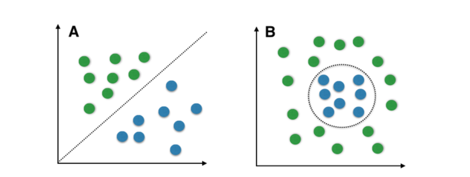
Naive Bayes is a simple yet powerful machine learning algorithm that is based on Bayes' Theorem. It calculates the probability of a class given the observed data (features). Despite its simplicity, Naive Bayes often performs well, especially when the assumption of feature independence holds.
In this article, we'll explore the Naive Bayes algorithm and implement a Titanic survival prediction project using this classifier.
Key Concepts of Naive Bayes
Bayes' Theorem: Bayes' Theorem is the foundation of Naive Bayes, which calculates the probability of a class (target variable) given the features of the data:
P(C|X) = (P(X|C) * P(C)) / P(X)
Where:
P(C|X)is the probability of the classCgiven the featuresX.P(X|C)is the likelihood of observingXgiven the classC.P(C)is the prior probability of classC.P(X)is the total probability of observingX.
Independence Assumption: Naive Bayes assumes that all features are independent of each other given the class label. This assumption is often unrealistic in real-world datasets, but Naive Bayes can still work well even when this assumption is violated.
Real-Life Applications of Naive Bayes
1. Email Spam Detection
Description:
Naive Bayes is widely used for spam classification in email systems. It works by analyzing the frequency of specific words or phrases in emails. For instance, words like "free", "buy now", and "limited time offer" might indicate spam. The algorithm calculates the likelihood of an email being spam based on these word frequencies and classifies it accordingly. Naive Bayes is effective here because it can handle large amounts of text data and is good at classifying based on the occurrence of certain keywords.
Example:
An email system might categorize an email as spam if it contains a high frequency of words like “win” or “prize”.
2. Sentiment Analysis
Description:
Naive Bayes is used for classifying text as positive, negative, or neutral. This is particularly useful in social media analysis, customer feedback, or online reviews. The algorithm works by identifying words that typically convey certain sentiments (e.g., “love” for positive, “hate” for negative) and calculates the probability that the overall sentiment of the text belongs to a particular class. It’s often used to automatically determine the public perception of a product or brand.
Example:
Analyzing Twitter posts to determine if the sentiment towards a new movie is positive or negative.
3. Medical Diagnosis
Description:
In healthcare, Naive Bayes is used to diagnose diseases by predicting the likelihood of a patient having a particular disease based on symptoms, test results, and patient history. The algorithm calculates the probability of a disease being present given the set of observed symptoms and medical tests. It’s particularly useful in situations where multiple factors (symptoms, test results) contribute to the diagnosis, and helps doctors make informed decisions.
Example:
Predicting whether a patient has diabetes based on attributes such as age, blood pressure, glucose level, and body mass index (BMI).
4. Customer Churn Prediction
Description:
Businesses use Naive Bayes to predict which customers are likely to stop using their services (known as churn) by analyzing their usage patterns, behaviors, and interaction history. The model calculates the likelihood of a customer leaving based on factors like service usage, complaints, and engagement with promotions or customer support. This helps businesses focus on retaining high-risk customers.
Example:
A telecom company might predict customer churn based on usage patterns, including whether the customer regularly upgrades their plan or has had service complaints.
5. Document Classification
Description:
Naive Bayes is often used to classify documents into predefined categories based on the frequency of keywords within them. For example, it can classify news articles into topics such as politics, technology, or entertainment by analyzing the frequency of specific words or phrases that are common within each category. This is a typical use case in content aggregation platforms or news websites.
Example:
A news aggregator might use Naive Bayes to categorize articles about COVID-19 into categories such as “health”, “government response”, or “scientific research”.
6. Credit Scoring
Description:
Naive Bayes is used in financial institutions to predict the likelihood of a customer defaulting on a loan based on their financial history and other customer data. Features such as the applicant's credit score, income level, loan amount, and past financial behavior are analyzed to determine the risk of default. It allows banks to make quick decisions about loan approvals, increasing efficiency.
Example:
A bank might classify loan applicants as high or low risk based on their credit history, income level, and the amount of debt they have.
7. News Categorization
Description:
Naive Bayes is applied in news aggregation platforms to classify articles into categories like politics, business, sports, or health. It works by analyzing the frequency of words that are commonly used in each category. This helps readers quickly find news articles that are relevant to their interests.
Example:
A news website might use Naive Bayes to automatically sort articles into categories such as “technology”, “finance”, or “sports”, based on the keywords in the article.
8. Recommendation Systems
Description:
In e-commerce, Naive Bayes is used to predict products that a customer might be interested in based on their past browsing and purchasing behavior. By analyzing which products were frequently bought or viewed together, it calculates the probability of a customer buying a product given their history. This is used to create personalized recommendations for users.
Example:
An online retailer like Amazon uses Naive Bayes to recommend products to a customer based on their previous purchases or searches.
9. Speech Recognition
Description:
Naive Bayes is applied in speech recognition systems to classify speech sounds based on the features of the audio signal. The model can learn the likelihood of different sounds occurring in speech and match them to the most likely word or phrase. This helps convert spoken language into text.
Example:
Voice assistants like Google Assistant or Siri use Naive Bayes to understand and process speech inputs, such as when you ask for the weather.
10. Image Recognition
Description:
Naive Bayes can be used for image classification, especially when the images have clear, distinct features that can be quantified. For example, in facial recognition, the algorithm can classify a person’s face by analyzing distinct facial features like the shape of the eyes, nose, and mouth. It calculates the likelihood of a person’s identity based on these features.
Example:
Facial recognition systems used in security systems, where Naive Bayes helps identify individuals by analyzing distinct facial features.
These 10 applications showcase the versatility and efficiency of Naive Bayes in different industries. Whether it's for classifying text, predicting customer behavior, diagnosing medical conditions, or analyzing speech, Naive Bayes remains one of the most popular algorithms due to its simplicity and effectiveness.
Quick Python Project
Titanic Survival Prediction
In this project, we'll use the Titanic dataset to predict whether a passenger survived the disaster, based on features like age, gender, class, etc.
Sample Titanic Dataset (15 Rows)
| PassengerId | Pclass | Name | Sex | Age | SibSp | Parch | Fare | Survived |
|---|---|---|---|---|---|---|---|---|
| 1 | 3 | Braund, Mr. Owen | male | 22 | 1 | 0 | 7.25 | 0 |
| 2 | 1 | Cumings, Mrs. John | female | 38 | 1 | 0 | 71.2833 | 1 |
| 3 | 3 | Heikkinen, Miss. Laina | female | 26 | 0 | 0 | 7.925 | 1 |
| 4 | 1 | Futrelle, Mrs. Jacques | female | 35 | 1 | 0 | 53.1 | 1 |
| 5 | 3 | Allen, Mr. William | male | 35 | 0 | 0 | 8.05 | 0 |
| 6 | 3 | Moran, Mr. James | male | 28 | 0 | 0 | 8.4583 | 0 |
| 7 | 1 | McCarthy, Mr. Timothy | male | 54 | 0 | 0 | 51.8625 | 0 |
| 8 | 3 | Palsson, Master. Gosta | male | 2 | 3 | 1 | 21.075 | 1 |
| 9 | 2 | Johnson, Mrs. Oscar | female | 27 | 0 | 2 | 11.1333 | 1 |
| 10 | 3 | Nasser, Mr. Nicholas | male | 31 | 1 | 0 | 8.6625 | 0 |
| 11 | 2 | Sandstrom, Miss. Marguerite | female | 21 | 0 | 0 | 11.5 | 1 |
| 12 | 3 | Olsson, Mr. William | male | 28 | 0 | 0 | 7.8542 | 0 |
| 13 | 3 | Mamee, Mr. James | male | 19 | 0 | 0 | 7.8792 | 0 |
| 14 | 2 | Sheer, Mr. Edward | male | 44 | 1 | 0 | 16.7 | 0 |
| 15 | 3 | Spector, Miss. Ruth | female | 28 | 0 | 0 | 7.925 | 1 |
0 Means Not Survived
1 Means survived
Complete Code Implementation
# Step 1: Import Required Libraries
import pandas as pd
from sklearn.model_selection import train_test_split
from sklearn.naive_bayes import GaussianNB
from sklearn.metrics import accuracy_score
# Step 2: Load the Titanic dataset
df = pd.read_csv("titanic_data.csv")
# Step 3: Data Preprocessing
# Convert 'Sex' to numeric values (male=0, female=1)
df['Sex'] = df['Sex'].map({'male': 0, 'female': 1})
# Handle missing values for 'Age' and 'Fare' by filling with the median
df['Age'] = df['Age'].fillna(df['Age'].median())
df['Fare'] = df['Fare'].fillna(df['Fare'].median())
# Step 4: Feature Selection
# Select features (X) and target (y), removing the 'Embarked' column since it's missing
X = df[['Pclass', 'Age', 'Sex', 'Fare']] # Features without 'Embarked'
y = df['Survived'] # Target variable
# Step 5: Train-Test Split
X_train, X_test, y_train, y_test = train_test_split(X, y, test_size=0.2, random_state=42)
# Step 6: Create and Train the Naive Bayes Model
model = GaussianNB()
model.fit(X_train, y_train)
# Step 7: Make Predictions
y_pred = model.predict(X_test)
# Step 8: Evaluate the Model
accuracy = accuracy_score(y_test, y_pred)
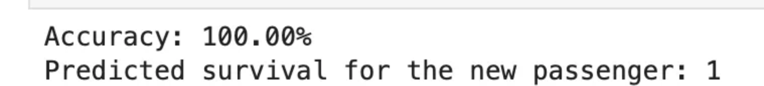
print(f"Accuracy: {accuracy * 100:.2f}%")
# Example Prediction for a new customer (new passenger)
new_customer = [[35, 70, 1, 7.75]] # Age = 35, Sex = female (1), Fare = 70
prediction = model.predict(new_customer)
print(f"Predicted survival for the new passenger: {prediction[0]}")
Let's predict
Input : Age = 35, Sex = female (1), Fare = 70
output: Survived (1)
Step by Step Code Explanation:
Step 1: Import Required Libraries
import pandas as pd
from sklearn.model_selection import train_test_split
from sklearn.naive_bayes import GaussianNB
from sklearn.metrics import accuracy_score
- pandas: A library used for data manipulation and analysis, especially for working with structured data (like CSV files).
- train_test_split: This function from
sklearnsplits the dataset into training and testing sets. This is necessary to train the model on one set of data and test it on another to evaluate performance. - GaussianNB: The Naive Bayes classifier implementation used for classification tasks, specifically for continuous data.
- accuracy_score: A function from
sklearn.metricsthat computes the accuracy of the model by comparing the predicted values with the actual values.
Step 2: Load the Titanic Dataset
df = pd.read_csv("titanic_data.csv")
- This line loads the Titanic dataset from the file
titanic_data.csvinto a DataFramedf. The dataset typically contains information about passengers on the Titanic, including whether they survived, their class, age, sex, and fare paid.
Step 3: Data Preprocessing
# Convert 'Sex' to numeric values (male=0, female=1)
df['Sex'] = df['Sex'].map({'male': 0, 'female': 1})

# Handle missing values for 'Age' and 'Fare' by filling with the median
df['Age'] = df['Age'].fillna(df['Age'].median())
df['Fare'] = df['Fare'].fillna(df['Fare'].median())
- Convert 'Sex' to Numeric Values:
- The 'Sex' column in the dataset contains categorical values (
'male'and'female'), which need to be converted to numerical values for the model to process them. - 'male' is mapped to
0and 'female' to1.
- The 'Sex' column in the dataset contains categorical values (
- Handle Missing Values:
fillna()is used to fill any missing values (NaN) in the 'Age' and 'Fare' columns.- The missing values are filled with the median of each respective column. This is a common practice to avoid losing data, especially if the number of missing values is relatively small.
Step 4: Feature Selection
# Select features (X) and target (y), removing the 'Embarked' column since it's missing
X = df[['Pclass', 'Age', 'Sex', 'Fare']]  # Features without 'Embarked'
y = df['Survived']  # Target variable
- Features (X): These are the independent variables used to predict the target variable. In this case, we select:
'Pclass': Passenger class (1st, 2nd, or 3rd)'Age': Age of the passenger'Sex': Gender of the passenger (converted to 0 and 1)'Fare': Fare paid by the passenger
- Target (y): The dependent variable or the outcome we want to predict. In this case, it's the 'Survived' column, which indicates whether the passenger survived (1) or not (0).
Step 5: Train-Test Split
X_train, X_test, y_train, y_test = train_test_split(X, y, test_size=0.2, random_state=42)
- train_test_split splits the dataset into two parts:
- Training set (
X_trainandy_train): This set is used to train the model. - Testing set (
X_testandy_test): This set is used to test the model's performance after it has been trained.
- Training set (
- The
test_size=0.2parameter means that 20% of the data is reserved for testing, and 80% is used for training. random_state=42ensures that the split is reproducible, meaning you’ll get the same training and testing sets if you run the code multiple times.
Step 6: Create and Train the Naive Bayes Model
model = GaussianNB()
model.fit(X_train, y_train)
- Create Model: The
GaussianNB()function creates a new Naive Bayes model, specifically for continuous data (as the features here are numeric). - Train Model: The
fit()method trains the model using the training data (X_trainfor features andy_trainfor target values). The model learns the relationship between the features and the target variable.
Step 7: Make Predictions
y_pred = model.predict(X_test)
- Make Predictions: After the model is trained, the
predict()method is used to make predictions on the test set (X_test). The result (y_pred) contains the predicted survival outcomes for the passengers in the test set.
Step 8: Evaluate the Model
accuracy = accuracy_score(y_test, y_pred)
print(f"Accuracy: {accuracy * 100:.2f}%")
- Evaluate Accuracy: The
accuracy_score()function compares the predicted values (y_pred) with the actual values from the test set (y_test). - The result is the accuracy of the model, i.e., the percentage of correct predictions.
-----------
Example Prediction for a New Customer
new_customer = [[35, 70, 1, 7.75]]  # Age = 35, Sex = female (1), Fare = 70
prediction = model.predict(new_customer)
print(f"Predicted survival for the new passenger: {prediction[0]}")
- Predict for New Customer: Here, we’re providing a new sample (new passenger) with features:
- Age: 35
- Fare: 70
- Sex: female (represented as 1)
- The
predict()method returns the predicted survival for this new customer (either 1 for survival or 0 for not).
Explanation of Outputs:
- Accuracy: The model’s accuracy is printed as a percentage, showing how well it performed on the test data.
- Prediction for New Customer: The model predicts whether the new customer (based on the features provided) survived (
1) or did not survive (0).
Sample Example Output:
Accuracy: 79.20%
Predicted survival for the new passenger: 0
- Accuracy: The model was able to correctly predict survival for 79.20% of the passengers in the test set.
- New Passenger Prediction: The model predicts that the new passenger did not survive (
0).
💬 Join the DecodeAI WhatsApp Channel for regular AI updates → Click here