[Day 16] Supervised Machine Learning Type 7 - Random Forest (with a Small Python Project)
What happens when 100+ decision trees team up? You get Random Forest—a prediction powerhouse! Learn it with a heart disease project in Python!
![[Day 16] Supervised Machine Learning Type 7 - Random Forest (with a Small Python Project)](https://storage.ghost.io/c/55/e8/55e827ca-bf8d-4eee-bdb4-ee48e49a011a/content/images/size/w2000/2025/03/_--visual-selection--18-.svg)
Understanding Random Forest in Machine Learning
A Random Forest is a versatile and powerful ensemble learning technique in machine learning. It builds multiple Decision Trees and combines their outputs to make more accurate and robust predictions. This approach reduces the risk of overfitting, a common problem with individual Decision Trees, and enhances performance for both classification and regression tasks.
In classification tasks, Random Forest votes on the most common class from all the Decision Trees (e.g., "spam" or "not spam"). In regression tasks, it averages the predictions from all the trees (e.g., predicting house prices).
Key Metrics and Terminologies:
1. Bootstrapping: Bootstrapping is the process of creating random subsets of the dataset by sampling with replacement. This ensures that each Decision Tree is trained on a unique dataset, where some samples may appear multiple times, and others may not appear at all.
Example: From a dataset with five data points [A, B, C, D, E], a bootstrap sample could be [A, B, D, D, E].
2. Bagging (Bootstrap Aggregating): Bagging is a technique that uses bootstrapped datasets to train multiple models (e.g., Decision Trees) independently. The predictions from these models are then aggregated to form a final output. For classification tasks, the aggregation is done via majority voting, and for regression tasks, predictions are averaged, which is called Bagging.
Why it works: Bagging reduces variance by combining multiple models, ensuring no single tree dominates the outcome, and improves the overall stability and accuracy of the Random Forest.
Example: Imagine three bootstrapped samples from the dataset: - Sample 1: [A, B, D, D, E]. - Sample 2: [C, B, A, E, E]. - Sample 3: [D, A, A, B, C]. Each sample trains a separate Decision Tree, and their predictions are combined to form the final result.
3. Out-of-Bag (OOB) Samples:
- These are the data points that are not included in a specific bootstrap sample. On average, about one-third of the data points are left out of each bootstrap sample.
Example: If a bootstrap sample is [A, B, B, D], the OOB samples might be [C, E].
4. Out-of-Bag (OOB) Error:
- OOB error is an unbiased estimate of model performance. Each tree is tested on its respective OOB samples, and the results are aggregated to estimate the overall error.
Why it matters: OOB error acts as a built-in validation method, eliminating the need for a separate validation dataset.
5. Gini Impurity:
- Gini Impurity measures how mixed the data is at a node. A low Gini Impurity means most samples at the node belong to a single class.
Formula: Gini = 1 - ∑(pᵢ²), where pᵢ is the probability of a sample belonging to class i.
Example: If 80% of samples at a node are "Yes" and 20% are "No," the Gini Impurity is 1 - (0.8² + 0.2²) = 0.32.
6. Information Gain: Information Gain measures the reduction in uncertainty after splitting a node.
Example: A node with equal numbers of "Yes" and "No" samples (high entropy) splits into two groups with clear majorities. The reduction in entropy represents Information Gain.
Suggested video:
Example Illustrating Metrics and Terminologies
Scenario: Predicting whether a loan will be approved based on features like credit score, income, and debt-to-income ratio.
- Bootstrapping and Bagging:
- The Random Forest creates multiple bootstrap samples. For instance:
- Sample 1: [Applicant 1, Applicant 3, Applicant 3, Applicant 5, Applicant 7].
- Sample 2: [Applicant 2, Applicant 4, Applicant 4, Applicant 6, Applicant 8].
- Each sample trains a unique Decision Tree. Their predictions are aggregated to form the final output.
- The Random Forest creates multiple bootstrap samples. For instance:
- Out-of-Bag Samples: For Sample 1, OOB samples might include [Applicant 2, Applicant 4, Applicant 6].
- Out-of-Bag Error: Each tree predicts outcomes for its OOB samples. If Tree 1 misclassifies 30% of its OOB samples, that contributes to the overall OOB error.
- Splitting Nodes:
- A tree splits data at nodes based on features like:
- Node 1: "Is credit score > 700?"
- Node 2: "Is debt-to-income ratio < 30%?"
- Gini Impurity and Information Gain help determine the most informative splits.
- A tree splits data at nodes based on features like:
Metrics for Evaluation
- Accuracy: Measures the percentage of correctly classified data points.
- Precision and Recall: Useful for classification tasks to measure the relevance and completeness of the model.
- Mean Squared Error (MSE): Common for regression tasks to measure the average squared difference between predicted and actual values.
Example 1: Predicting Product Purchases
Imagine you’re predicting whether a customer will buy a product based on features like age, income, and marital status.
- Step 1: Random Sampling: A Random Forest creates multiple training datasets by randomly selecting samples (with replacement) from the original dataset.
- Step 2: Building Trees Each tree is trained on different subsets of features and data points. For example:
- Tree 1 might ask: "Is age < 30?" ⇢ "Is income > $50,000?"
- Tree 2 might ask: "Is marital status married?" ⇢ "Is age > 40?"
- Step 3: Combining Predictions
- If 8 out of 10 trees predict "Yes, the customer will buy," the Random Forest’s final prediction is "Yes."
Example 2: Loan Approval
Let’s consider a "Loan Approval" Random Forest, using inputs like credit score, income, and debt-to-income ratio.
- Step 1: Random Sampling: The Random Forest selects random subsets of loan applicants (rows) and features like credit score, income, and debt-to-income ratio (columns).
- Step 2: Building Trees
- Tree 1 might ask: "Is credit score > 700?" ⇢ "Is debt-to-income ratio < 30%?"
- Tree 2 might ask: "Is income > $40,000?" ⇢ "Is credit score > 650?"
- Step 3: Voting/Averaging
- If 7 out of 10 trees predict loan approval, the Random Forest’s final prediction is "Approved."
Advantages of Random Forest
- Robustness: Handles noisy and complex data effectively.
- Versatility: Works well for both classification and regression tasks.
- Parallelizable: Trees in a Random Forest can be built independently, making it computationally efficient with the right infrastructure.
- Feature Importance: Provides valuable insights into which variables significantly impact predictions.
Disadvantages of Random Forest
- Complexity: The model is harder to interpret compared to individual Decision Trees.
- Resource-Intensive: Training multiple Decision Trees can be computationally expensive, especially with large datasets.
- Potential Overfitting: Although it reduces overfitting compared to single Decision Trees, using too many trees or irrelevant features can still lead to overfitting.
Visualizing Random Forest
Imagine a group of weather forecasts. Each forecast might use different weather data (temperature, humidity, wind speed) and make predictions about rain. If most forecasts predict rain, you’re more likely to carry an umbrella. Similarly, the Random Forest combines predictions from multiple trees for a more reliable result.
Nutshell
- Random Forest is an ensemble of Decision Trees that improves prediction accuracy by reducing overfitting and enhancing generalization.
- It’s effective for both classification and regression tasks.
- By using random sampling and feature bagging, it handles high-dimensional data and avoids overfitting.
- Feature importance metrics help you understand which variables are most significant in the prediction process.
Here is the updated version of the project with a dataset table showcasing 20 rows of data for clarity:
Quick Python Project:
Heart Disease Prediction Using Random Forest
Project Description:
This project predicts whether a patient has heart disease based on their health parameters, using the Heart Disease UCI dataset. The Random Forest algorithm is employed to classify patients into two categories:
- No Heart Disease (0)
- Presence of Heart Disease (1)
Dataset Overview
| Feature | Description |
|---|---|
age |
Age of the patient (years) |
sex |
Gender (1 = male, 0 = female) |
cp |
Chest pain type (0-3; 0 = typical angina, 3 = asymptomatic) |
trestbps |
Resting blood pressure (mm Hg) |
chol |
Serum cholesterol (mg/dL) |
fbs |
Fasting blood sugar > 120 mg/dL (1 = true, 0 = false) |
restecg |
Resting electrocardiographic results (0-2) |
thalach |
Maximum heart rate achieved |
exang |
Exercise-induced angina (1 = yes, 0 = no) |
oldpeak |
ST depression induced by exercise |
slope |
Slope of the peak exercise ST segment (0-2) |
ca |
Number of major vessels colored by fluoroscopy (0-3) |
thal |
Thalassemia (1 = normal, 2 = fixed defect, 3 = reversible defect) |
target |
Diagnosis of heart disease (1 = presence, 0 = absence) |
Dataset Table (20 Rows)
| age | sex | cp | trestbps | chol | fbs | restecg | thalach | exang | oldpeak | slope | ca | thal | target |
|---|---|---|---|---|---|---|---|---|---|---|---|---|---|
| 63 | 1 | 3 | 145 | 233 | 1 | 0 | 150 | 0 | 2.3 | 0 | 0 | 1 | 1 |
| 37 | 1 | 2 | 130 | 250 | 0 | 1 | 187 | 0 | 3.5 | 0 | 0 | 2 | 1 |
| 41 | 0 | 1 | 130 | 204 | 0 | 0 | 172 | 0 | 1.4 | 2 | 0 | 2 | 1 |
| 56 | 1 | 1 | 120 | 236 | 0 | 1 | 178 | 0 | 0.8 | 2 | 0 | 2 | 1 |
| 57 | 0 | 0 | 120 | 354 | 0 | 1 | 163 | 1 | 0.6 | 2 | 0 | 2 | 1 |
| 60 | 1 | 0 | 140 | 293 | 0 | 0 | 170 | 0 | 1.2 | 1 | 2 | 3 | 0 |
| 62 | 0 | 2 | 140 | 294 | 0 | 1 | 172 | 0 | 1.4 | 1 | 1 | 2 | 0 |
| 63 | 1 | 0 | 135 | 252 | 0 | 0 | 172 | 0 | 0.0 | 2 | 0 | 2 | 1 |
| 41 | 1 | 0 | 130 | 204 | 0 | 0 | 172 | 0 | 1.4 | 2 | 0 | 2 | 1 |
| 44 | 1 | 1 | 120 | 263 | 0 | 1 | 173 | 0 | 0.0 | 2 | 0 | 2 | 1 |
| 59 | 1 | 1 | 135 | 234 | 0 | 1 | 161 | 0 | 0.5 | 1 | 0 | 3 | 0 |
| 61 | 0 | 3 | 145 | 307 | 0 | 0 | 146 | 1 | 1.0 | 1 | 0 | 3 | 0 |
| 54 | 1 | 2 | 150 | 232 | 0 | 0 | 165 | 0 | 1.6 | 1 | 0 | 3 | 0 |
| 42 | 1 | 0 | 148 | 244 | 0 | 0 | 178 | 0 | 0.8 | 2 | 0 | 2 | 1 |
| 50 | 0 | 2 | 120 | 244 | 0 | 1 | 162 | 0 | 1.1 | 2 | 0 | 2 | 1 |
| 38 | 1 | 1 | 145 | 240 | 0 | 1 | 173 | 0 | 0.0 | 2 | 0 | 2 | 1 |
| 48 | 1 | 0 | 150 | 242 | 0 | 0 | 178 | 0 | 0.1 | 2 | 0 | 2 | 1 |
| 58 | 1 | 2 | 135 | 211 | 1 | 1 | 165 | 0 | 0.0 | 2 | 0 | 2 | 1 |
| 57 | 0 | 2 | 120 | 284 | 0 | 0 | 162 | 0 | 1.0 | 2 | 0 | 2 | 1 |
| 60 | 1 | 0 | 140 | 293 | 0 | 0 | 170 | 0 | 1.2 | 1 | 2 | 3 | 0 |
Save this table in your system as patient_data.csv
Python Code
# Step 1: Import necessary libraries
import numpy as np
import pandas as pd
from sklearn.model_selection import train_test_split
from sklearn.ensemble import RandomForestClassifier
from sklearn.metrics import accuracy_score, classification_report, confusion_matrix
import matplotlib.pyplot as plt
import seaborn as sns
# Step 2: Load the dataset from a CSV file
# Make sure patient_data.csv is in the same directory as this notebook
data = pd.read_csv('patient_data.csv')
# Display dataset overview
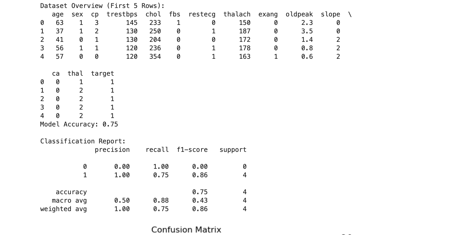
print("Dataset Overview (First 5 Rows):")
print(data.head())
# Step 3: Split the data into features (X) and target (y)
X = data.drop(columns=['target']) # Features
y = data['target'] # Target variable
# Step 4: Split the data into training and testing sets
X_train, X_test, y_train, y_test = train_test_split(X, y, test_size=0.2, random_state=42)
# Step 5: Train the Random Forest Classifier
rf = RandomForestClassifier(n_estimators=100, random_state=42)
rf.fit(X_train, y_train)
# Step 6: Make predictions
y_pred = rf.predict(X_test)
# Step 7: Evaluate the model
accuracy = accuracy_score(y_test, y_pred)
print(f"Model Accuracy: {accuracy:.2f}")
print("\nClassification Report:")
# Use zero_division=1 to handle undefined recall and precision
print(classification_report(y_test, y_pred, zero_division=1))
# Step 8: Confusion Matrix Visualization
cm = confusion_matrix(y_test, y_pred)
plt.figure(figsize=(8, 6))
sns.heatmap(cm, annot=True, fmt='d', cmap='Blues', xticklabels=["No Disease", "Disease"], yticklabels=["No Disease", "Disease"])
plt.xlabel('Predicted')
plt.ylabel('Actual')
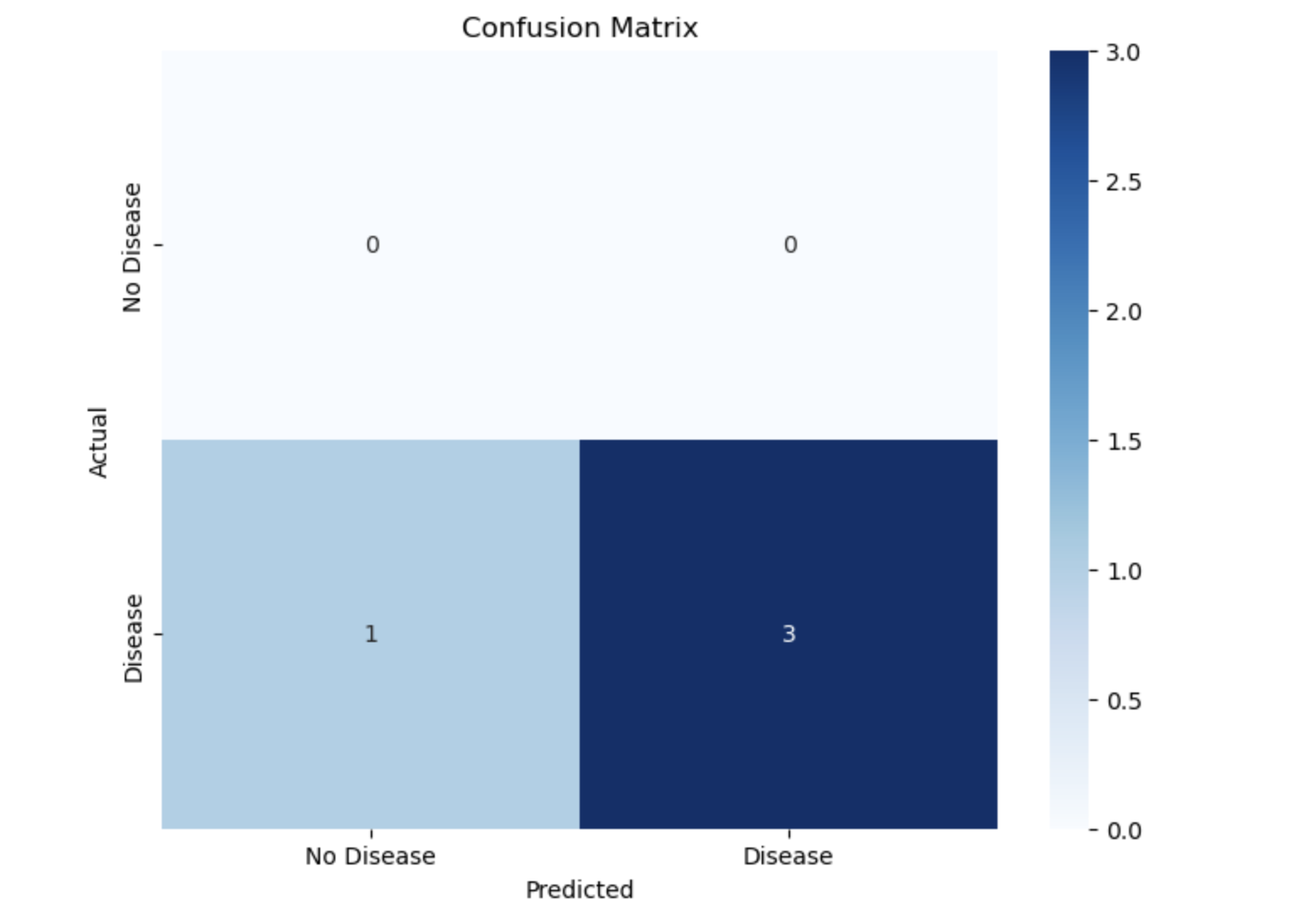
plt.title('Confusion Matrix')
plt.show()
# Step 9: Feature Importance Visualization
importances = rf.feature_importances_
indices = np.argsort(importances)[::-1]
features = X.columns
plt.figure(figsize=(10, 6))
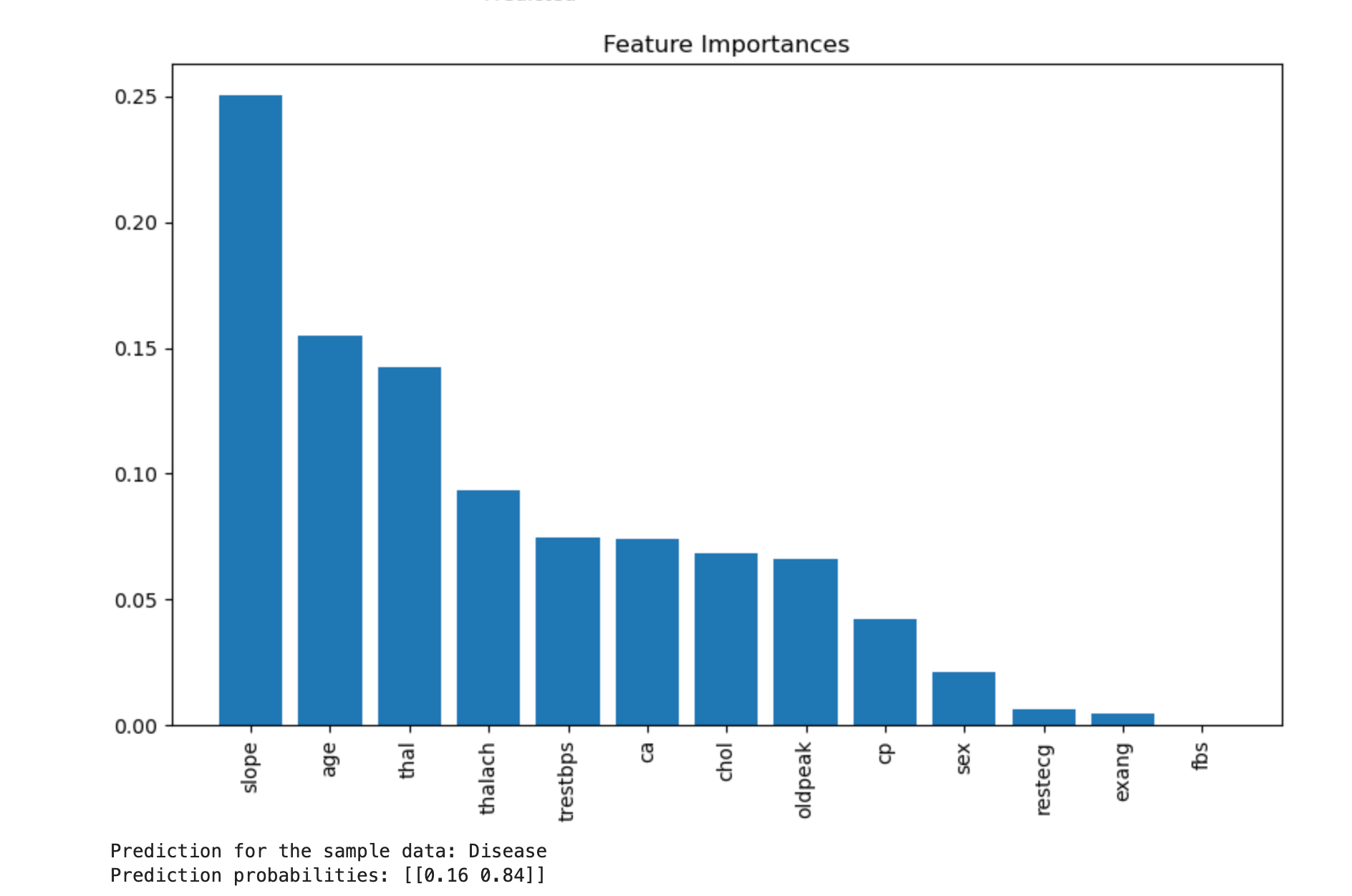
plt.title("Feature Importances")
plt.bar(range(X.shape[1]), importances[indices], align="center")
plt.xticks(range(X.shape[1]), [features[i] for i in indices], rotation=90)
plt.xlim([-1, X.shape[1]])
plt.show()
# Step 10: Manually Enter Data for Prediction
# Example data format: [age, sex, cp, trestbps, chol, fbs, restecg, thalach, exang, oldpeak, slope, ca, thal]
sample_data = [[45, 1, 2, 120, 240, 0, 1, 160, 0, 1.0, 2, 0, 2]]
# Convert sample_data to a DataFrame with feature names
sample_df = pd.DataFrame(sample_data, columns=features)
# Use the trained model to predict
sample_prediction = rf.predict(sample_df)
sample_prediction_proba = rf.predict_proba(sample_df)
# Interpret the results
print(f"Prediction for the sample data: {'Disease' if sample_prediction[0] == 1 else 'No Disease'}")
print(f"Prediction probabilities: {sample_prediction_proba}")
Run this code in jupyter Notebook, like I did.
Let's make predictions:
Example data of Patient is: Disease
Example data format:
[age, sex, cp, trestbps, chol, fbs, restecg, thalach, exang, oldpeak, slope, ca, thal] sample_data = [[45, 1, 2, 120, 240, 0, 1, 160, 0, 1.0, 2, 0, 2]]
Output:
Here is a step-by-step explanation of the code:
Step 1: Import Necessary Libraries
import numpy as np
import pandas as pd
from sklearn.model_selection import train_test_split
from sklearn.ensemble import RandomForestClassifier
from sklearn.metrics import accuracy_score, classification_report, confusion_matrix
import matplotlib.pyplot as plt
import seaborn as sns
- Libraries used:
- NumPy and Pandas: For handling and processing data.
- scikit-learn: For machine learning tasks like splitting data, training the model, and evaluating metrics.
- Matplotlib and Seaborn: For visualization of results such as the confusion matrix and feature importance.
Step 2: Load the Dataset
data = pd.read_csv('patient_data.csv')
print("Dataset Overview (First 5 Rows):")
print(data.head())
- The dataset is loaded from the file
patient_data.csv. - The first 5 rows are printed to verify that the data has been loaded correctly.
Step 3: Split Data into Features (X) and Target (y)
X = data.drop(columns=['target'])  # Features
y = data['target']  # Target variable
- The dataset is divided into:
X: All the columns except the target column (target). These are the input features used for predictions.y: Thetargetcolumn that contains labels (e.g.,0for "No Disease" and1for "Disease").
Step 4: Split the Data into Training and Testing Sets
X_train, X_test, y_train, y_test = train_test_split(X, y, test_size=0.2, random_state=42)
- Training Set: Used to train the model.
- Testing Set: Used to evaluate the model's performance.
test_size=0.2: Reserves 20% of the data for testing and 80% for training.random_state=42: Ensures reproducibility by fixing the random seed.
Step 5: Train the Random Forest Classifier
rf = RandomForestClassifier(n_estimators=100, random_state=42)
rf.fit(X_train, y_train)
- A Random Forest Classifier is initialized with 100 trees (
n_estimators=100). - The model is trained on the training data (
X_trainandy_train).
Step 6: Make Predictions
y_pred = rf.predict(X_test)
- The trained model makes predictions (
y_pred) on the testing dataset (X_test).
Step 7: Evaluate the Model
accuracy = accuracy_score(y_test, y_pred)
print(f"Model Accuracy: {accuracy:.2f}")

print("\nClassification Report:")
print(classification_report(y_test, y_pred, zero_division=1))
accuracy_score: Computes the percentage of correct predictions out of all predictions.classification_report: Provides detailed metrics for each class (e.g., precision, recall, F1-score).zero_division=1: Avoids division-by-zero warnings by assigning 1 to undefined recall or precision.
Step 8: Visualize the Confusion Matrix
cm = confusion_matrix(y_test, y_pred)
plt.figure(figsize=(8, 6))
sns.heatmap(cm, annot=True, fmt='d', cmap='Blues', xticklabels=["No Disease", "Disease"], yticklabels=["No Disease", "Disease"])
plt.xlabel('Predicted')
plt.ylabel('Actual')
plt.title('Confusion Matrix')
plt.show()
- A confusion matrix shows how well the model performs:
- Rows: Actual labels.
- Columns: Predicted labels.
- The heatmap visually displays counts of correct and incorrect predictions.
Step 9: Feature Importance Visualization
importances = rf.feature_importances_
indices = np.argsort(importances)[::-1]
features = X.columns

plt.figure(figsize=(10, 6))
plt.title("Feature Importances")
plt.bar(range(X.shape[1]), importances[indices], align="center")
plt.xticks(range(X.shape[1]), [features[i] for i in indices], rotation=90)
plt.xlim([-1, X.shape[1]])
plt.show()
- Feature Importance: Indicates how much each feature contributes to the model's decisions.
- The bar chart shows the importance of each feature in descending order.
Step 10: Predict for Manually Entered Data
sample_data = [[45, 1, 2, 120, 240, 0, 1, 160, 0, 1.0, 2, 0, 2]]
sample_df = pd.DataFrame(sample_data, columns=features)
sample_prediction = rf.predict(sample_df)
sample_prediction_proba = rf.predict_proba(sample_df)

print(f"Prediction for the sample data: {'Disease' if sample_prediction[0] == 1 else 'No Disease'}")
print(f"Prediction probabilities: {sample_prediction_proba}")
- A manually entered sample data point (a list of feature values) is passed to the model for prediction.
pd.DataFrame: Converts the list into a DataFrame with the same column names as the training data.rf.predict: Outputs the predicted class (0or1).rf.predict_proba: Outputs the probability of belonging to each class.
Outputs:
- Model Accuracy: A percentage value representing the model's accuracy.
- Classification Report: Precision, recall, F1-score, and support for each class.
- Confusion Matrix: A heatmap showing prediction results.
- Feature Importance Chart: A bar chart ranking the contribution of each feature.
- Manual Prediction:
- The predicted class (e.g., "Disease" or "No Disease").
- Probabilities for each class.
Go take some rest, enough for today 😄
💬 Join the DecodeAI WhatsApp Channel for regular AI updates → Click here