[Day 19] Unsupervised Machine Learning Type 2 - Hierarchical Clustering (with a Small Python Project)
From borrower risk levels to cancer cells—hierarchical clustering builds a tree of insights! Dive in with a visual Python demo 🚀📊
![[Day 19] Unsupervised Machine Learning Type 2 - Hierarchical Clustering (with a Small Python Project)](https://storage.ghost.io/c/55/e8/55e827ca-bf8d-4eee-bdb4-ee48e49a011a/content/images/size/w2000/2025/03/Gradient-Boosting-Machines-machine-learning-algo---visual-selection--3-.svg)
🎯 What is Hierarchical Clustering?
Hierarchical Clustering is a clustering algorithm that groups similar data points based on hierarchy rather than a fixed number of clusters like K-Means. It builds a tree-like structure (dendrogram) to show how clusters are formed at different levels.
Example: Borrower Segmentation in Credit Risk Analysis
Imagine a bank that wants to segment borrowers based on their creditworthiness. The bank collects data on credit score, income, loan amount, interest rate, and repayment history.
🔹 Hierarchical Clustering helps!
- It groups borrowers into low-risk, medium-risk, and high-risk based on financial behavior.
- Borrowers in Cluster 0 have the highest credit scores and stable income.
- Borrowers in Cluster 1 have lower credit scores and higher loan defaults.
- Helps banks in loan approvals and risk assessment.
🛒 Real-World Use Cases of Hierarchical Clustering
1.Customer Segmentation (E-Commerce & Retail)
📌 Problem: A business wants to group customers based on their shopping preferences. 🎯 Hierarchical Clustering Solution:
- Creates a hierarchy of customer groups (e.g., Budget Shoppers → Mid-range Shoppers → Premium Shoppers).
- Helps businesses refine their marketing strategies.
2.Fraud Detection in Banking
📌 Problem: A bank needs to detect fraudulent transactions. 🎯 Hierarchical Clustering Solution:
- Groups transactions into low-risk, medium-risk, and high-risk based on spending patterns.
- Helps banks like JP Morgan and Citibank identify emerging fraud patterns.
3.Medical Research: Classifying Cancer Cells
📌 Problem: Doctors need to classify cancerous and non-cancerous cells. 🎯 Hierarchical Clustering Solution:
- Groups cells into healthy, pre-cancerous, and cancerous based on genetic similarities.
- Used in hospitals for early cancer detection.
📊 How Hierarchical Clustering Works (Step by Step)

Step 1: Start with Individual Clusters
- Each data point is initially treated as its own cluster.
Step 2: Merge the Closest Clusters
- The two most similar clusters are merged into one.
Step 3: Repeat Until One Big Cluster is Left
- This merging process continues until all points belong to a single cluster.
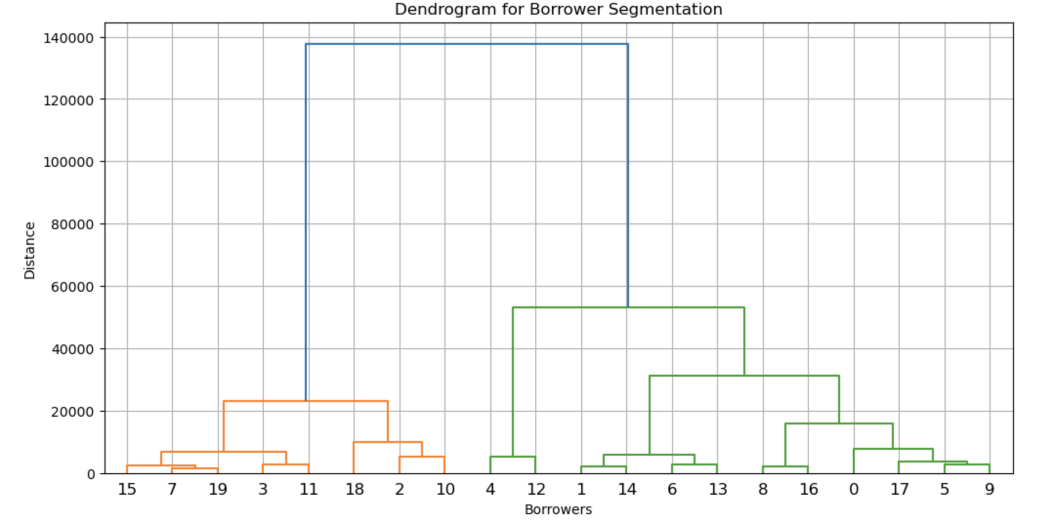
Step 4: Use the Dendrogram to Decide Clusters
- A dendrogram (tree diagram) is used to cut at the optimal level to form meaningful clusters.
🎯 Final Result: A hierarchy of clusters, allowing flexibility in choosing the number of groups.
🖥 Python Mini Project: Borrower Segmentation for Credit Risk
Let’s build a Hierarchical Clustering model to segment borrowers based on their credit profiles.
🔹 Dataset: borrower_data.csv
Save this table as borrower_data.csv
| Borrower ID | Credit Score | Income ($) | Loan Amount ($) | Interest Rate (%) | Repayment History (1-Default, 0-Good) |
|---|---|---|---|---|---|
| 1 | 750 | 90000 | 20000 | 5.5 | 0 |
| 2 | 680 | 75000 | 30000 | 7.0 | 0 |
| 3 | 620 | 50000 | 40000 | 9.5 | 1 |
| 4 | 580 | 45000 | 50000 | 11.0 | 1 |
| 5 | 800 | 110000 | 15000 | 4.0 | 0 |
| 6 | 720 | 85000 | 25000 | 6.0 | 0 |
| 7 | 690 | 78000 | 28000 | 6.5 | 0 |
| 8 | 610 | 48000 | 45000 | 10.0 | 1 |
| 9 | 770 | 96000 | 22000 | 5.0 | 0 |
| 10 | 730 | 87000 | 27000 | 5.8 | 0 |
| 11 | 640 | 55000 | 38000 | 9.0 | 1 |
| 12 | 590 | 47000 | 48000 | 10.5 | 1 |
| 13 | 810 | 115000 | 14000 | 3.8 | 0 |
| 14 | 700 | 80000 | 26000 | 6.2 | 0 |
| 15 | 680 | 77000 | 30000 | 6.8 | 0 |
| 16 | 605 | 49000 | 44000 | 9.8 | 1 |
| 17 | 785 | 98000 | 21000 | 4.8 | 0 |
| 18 | 740 | 89000 | 25000 | 5.5 | 0 |
| 19 | 655 | 60000 | 35000 | 8.5 | 1 |
| 20 | 610 | 47000 | 46000 | 10.2 | 1 |
📝 Python Code for Hierarchical Clustering (Borrower Segmentation)
import pandas as pd
import matplotlib.pyplot as plt
import seaborn as sns
import scipy.cluster.hierarchy as sch
from sklearn.cluster import AgglomerativeClustering

# Step 1: Load Dataset
data = pd.read_csv("borrower_data.csv")
X = data[['Credit Score', 'Income ($)', 'Loan Amount ($)', 'Interest Rate (%)', 'Repayment History']]

# Step 2: Create Dendrogram to Find Optimal Clusters
plt.figure(figsize=(12, 6))
dendrogram = sch.dendrogram(sch.linkage(X, method='ward'))
plt.xlabel('Borrowers')
plt.ylabel('Distance')
plt.title('Dendrogram for Borrower Segmentation')
plt.grid()
plt.show()

# Step 3: Apply Hierarchical Clustering
hc = AgglomerativeClustering(n_clusters=3, metric='euclidean', linkage='ward')
data['Cluster'] = hc.fit_predict(X)

# Step 4: Visualize Clusters in a Pairplot
sns.pairplot(data, hue='Cluster', palette='Set1')
plt.show()

# Step 5: Scatter Plot with Multiple Features
plt.figure(figsize=(10, 6))
sns.scatterplot(x=data['Credit Score'], y=data['Income ($)'], hue=data['Cluster'], palette='Set1', s=100)
plt.xlabel('Credit Score')
plt.ylabel('Income ($)')
plt.title('Borrower Segmentation using Hierarchical Clustering')
plt.legend(title='Cluster')
plt.grid()
plt.show()
Result:
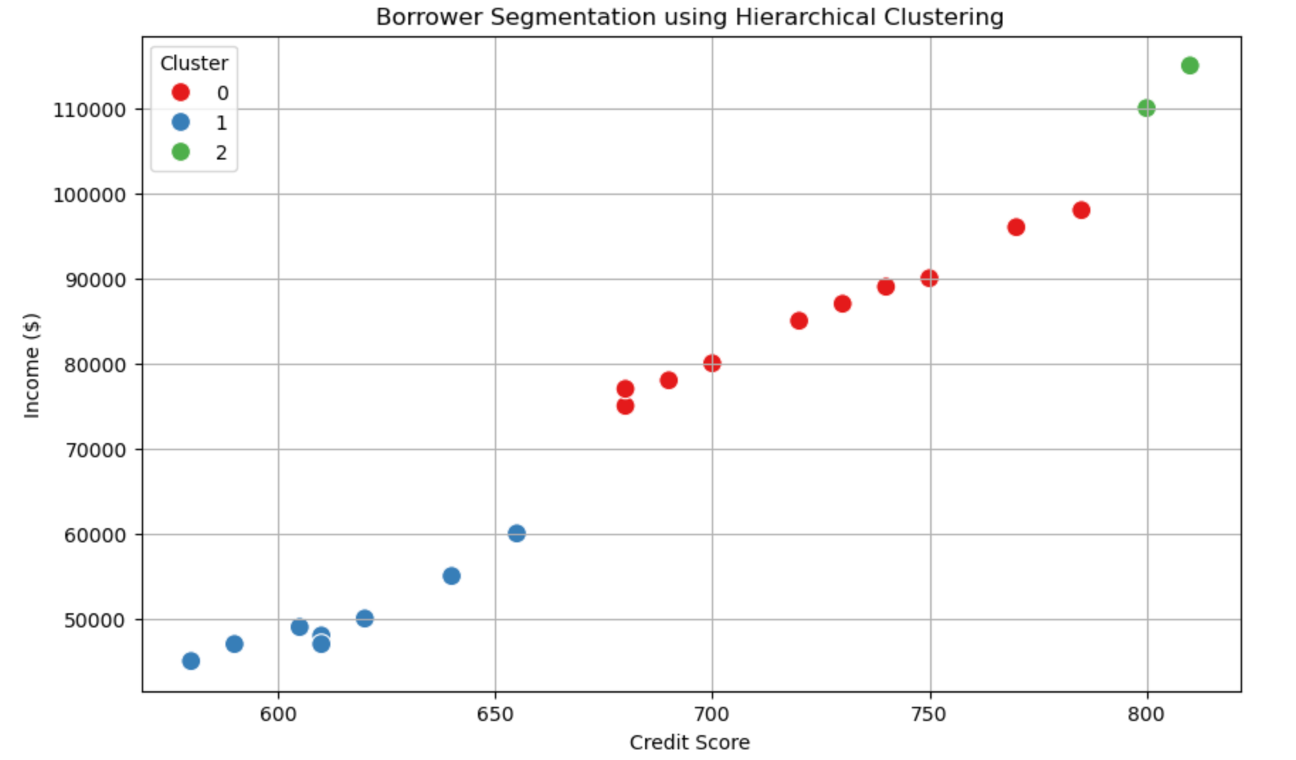
📊 Explanation of the Borrower Segmentation Chart
This scatter plot represents borrower segmentation using Hierarchical Clustering, where:
- X-axis (Credit Score): Represents the borrower's credit score (higher scores indicate better creditworthiness).
- Y-axis (Income $): Represents the annual income of the borrower.
- Color-coded Clusters: Each borrower is assigned to a cluster based on their financial characteristics.
🔹 Interpreting the Clusters
- Cluster 0 (Red Points - Medium-Risk Borrowers)
- Most borrowers in this cluster have moderate credit scores (650-750).
- They also have decent income levels but may not be the highest earners.
- These borrowers are likely to get loans but with slightly higher interest rates.
- Cluster 1 (Blue Points - High-Risk Borrowers)
- These borrowers have low credit scores (below 650) and lower income levels.
- They may have poor repayment history or high debt burdens.
- They are considered high-risk for banks, meaning they might either get denied loans or charged higher interest rates.
- Cluster 2 (Green Points - Low-Risk Borrowers)
- Borrowers in this cluster have very high credit scores (above 780).
- They also have higher income levels (above $100,000).
- These individuals are low-risk, meaning banks can offer them better loan terms with lower interest rates.
🎯 What Can We Conclude?
- Banks can use this segmentation to make loan approval decisions.
- Cluster 2 borrowers are the best candidates for loans.
- Cluster 1 borrowers need financial improvement before getting favorable loans.
- Cluster 0 borrowers fall somewhere in between and may receive standard loan terms.
This approach helps financial institutions optimize risk assessment while offering loans to different borrower profiles! 🚀
💡 Nutshell
✅ Hierarchical Clustering is useful when we don’t know the number of clusters in advance.
✅ It helps banks in credit risk assessment and loan approvals.
✅ It is widely used in banking, healthcare, and customer segmentation.
💬 Join the DecodeAI WhatsApp Channel for regular AI updates → Click here