[Day 20] Unsupervised Machine Learning Type 3 - DBSCAN (with a Small Python Project)
Forget fixed clusters—DBSCAN hunts down dense transaction zones and flags outliers like a fraud-sniffing detective. 🕵️♂️💳
![[Day 20] Unsupervised Machine Learning Type 3 - DBSCAN (with a Small Python Project)](https://storage.ghost.io/c/55/e8/55e827ca-bf8d-4eee-bdb4-ee48e49a011a/content/images/size/w2000/2025/03/Gradient-Boosting-Machines-machine-learning-algo---visual-selection--4-.svg)
What is DBSCAN?
DBSCAN stands for Density-Based Spatial Clustering of Applications with Noise. Unlike K-Means, which assumes clusters are spherical and require you to specify the number of clusters (K), DBSCAN finds clusters of arbitrary shapes based on how densely packed data points are. It’s also great at spotting outliers (noise) that don’t belong to any cluster.
Why is DBSCAN Important in Real Life?
- Fraud Detection: Identifies unusual transaction patterns that don’t fit normal clusters.
- Astronomy: Groups stars or galaxies based on their spatial density in the sky.
- Geographical Analysis: Detects hotspots like crime zones or disease outbreaks.
Let’s break it down simply!
What is DBSCAN Clustering?
DBSCAN groups data points that are close together (dense regions) into clusters, while marking sparse points as noise. It doesn’t need you to predefine the number of clusters—pretty cool, right?
DBSCAN groups data points that are close together (dense regions) into clusters, while marking sparse points as noise. It doesn’t need you to predefine the number of clusters—pretty cool, right? Unlike K-Means, which struggles with irregular shapes and forces every point into a cluster, DBSCAN is smarter about density. It only groups points that naturally belong together based on how tightly packed they are, leaving loners out in the cold as “noise.” This makes it a go-to choice when your data has messy, real-world patterns rather than neat, predefined categories. Think of it as a detective that finds the crowd and ignores the stragglers!
Example 1: Crime Hotspot Detection
Imagine a city that wants to identify crime hotspots using location data (latitude, longitude).
- DBSCAN steps in!
- It groups dense clusters of crime incidents into “hotspots.”
- Isolated incidents? Labeled as noise, not part of any cluster.
Example 2: Fraud Detection Based on Transaction Patterns
Imagine a bank that wants to detect fraudulent transactions. It analyzes multiple transaction-related features like:
- Transaction Amount
- Time of Transaction
- Location Variance
- Previous Fraud Involvement
- Device Fingerprint Score
🔹 DBSCAN helps!
- It identifies dense groups of normal transactions.
- Isolates outliers, which could indicate fraudulent or suspicious behavior.
- Perfect for detecting anomalies in finance, cybersecurity, or healthcare.
Few more Real-World Use Cases of DBSCAN
- Outlier Detection in Banking
- Problem: A bank wants to flag suspicious transactions.
- DBSCAN Solution: Normal transactions form dense clusters; rare, odd ones are flagged as noise.
- Social Media Trend Analysis
- Problem: A platform wants to find trending topics.
- DBSCAN Solution: Groups similar posts into clusters based on keyword density, ignoring random noise posts.
- Epidemiology
- Problem: Health officials need to track disease outbreaks.
- DBSCAN Solution: Clusters dense regions of infection cases, marking sparse cases as outliers.
How DBSCAN Works (Step by Step)

DBSCAN relies on two key parameters:
- Epsilon (ε): The maximum distance between two points to be considered neighbors.
- MinPts: The minimum number of points needed to form a dense region (cluster).
Here’s the process
- Pick a Point: Start with an unvisited data point.
- Check Neighbors: If it has at least MinPts neighbors within ε distance, it’s a core point—start a cluster!
- Expand the Cluster: Add all density-reachable points (neighbors within ε) to the cluster.
- Mark Noise: Points with fewer than MinPts neighbors are labeled as noise.
- Repeat: Move to the next unvisited point until all points are processed.
Final Result: Clusters of varying shapes and sizes, plus outliers identified!
🖥 Python
Mini Project: Detecting Transaction Anomalies using DBSCAN
Let’s build a DBSCAN model to detect abnormal transactions.
Save below file as transaction_data.csv
| Transaction ID | Amount ($) | Hour | Device Score | Prev Fraud (0/1) | Location Variance |
|---|---|---|---|---|---|
| 1 | 25 | 10 | 0.91 | 0 | 0.12 |
| 2 | 5100 | 23 | 0.35 | 1 | 1.89 |
| 3 | 75 | 21 | 0.88 | 0 | 0.15 |
| 4 | 200 | 2 | 0.41 | 0 | 0.55 |
| 5 | 1500 | 22 | 0.40 | 1 | 0.96 |
| 6 | 12 | 9 | 0.95 | 0 | 0.10 |
| 7 | 340 | 5 | 0.89 | 0 | 0.20 |
| 8 | 4600 | 1 | 0.30 | 1 | 1.70 |
| 9 | 95 | 14 | 0.93 | 0 | 0.18 |
| 10 | 2200 | 23 | 0.36 | 1 | 1.45 |
| 11 | 48 | 12 | 0.92 | 0 | 0.11 |
| 12 | 3100 | 3 | 0.32 | 1 | 1.80 |
| 13 | 85 | 18 | 0.87 | 0 | 0.22 |
| 14 | 170 | 11 | 0.90 | 0 | 0.25 |
| 15 | 2500 | 22 | 0.38 | 1 | 1.40 |
| 16 | 30 | 15 | 0.94 | 0 | 0.09 |
| 17 | 520 | 6 | 0.85 | 0 | 0.24 |
| 18 | 4000 | 4 | 0.31 | 1 | 1.55 |
| 19 | 65 | 20 | 0.93 | 0 | 0.16 |
| 20 | 2900 | 23 | 0.37 | 1 | 1.60 |
| 21 | 100 | 17 | 0.89 | 0 | 0.20 |
| 22 | 3500 | 0 | 0.29 | 1 | 1.75 |
| 23 | 80 | 13 | 0.86 | 0 | 0.19 |
| 24 | 40 | 7 | 0.94 | 0 | 0.12 |
| 25 | 2700 | 21 | 0.34 | 1 | 1.68 |
📝 Python Code for Hierarchical Clustering (Borrower Segmentation)
import pandas as pd
import matplotlib.pyplot as plt
import seaborn as sns
from sklearn.preprocessing import StandardScaler
from sklearn.cluster import DBSCAN
from sklearn.decomposition import PCA

# Step 1: Load Dataset
data = pd.read_csv("transaction_data.csv")
X = data[['Amount ($)', 'Hour', 'Device Score', 'Prev Fraud (0/1)', 'Location Variance']]

# Step 2: Normalize Data
scaler = StandardScaler()
X_scaled = scaler.fit_transform(X)

# Step 3: Apply DBSCAN
dbscan = DBSCAN(eps=0.9, min_samples=3)
data['Cluster'] = dbscan.fit_predict(X_scaled)

# Step 4: Visualize Clusters using PCA
pca = PCA(n_components=2)
components = pca.fit_transform(X_scaled)
data['PCA1'] = components[:, 0]
data['PCA2'] = components[:, 1]

plt.figure(figsize=(10, 6))
sns.scatterplot(data=data, x='PCA1', y='PCA2', hue='Cluster', palette='Set1', s=100)
plt.title('Transaction Anomaly Detection using DBSCAN (PCA Visualization)')
plt.grid()
plt.show()
Result:
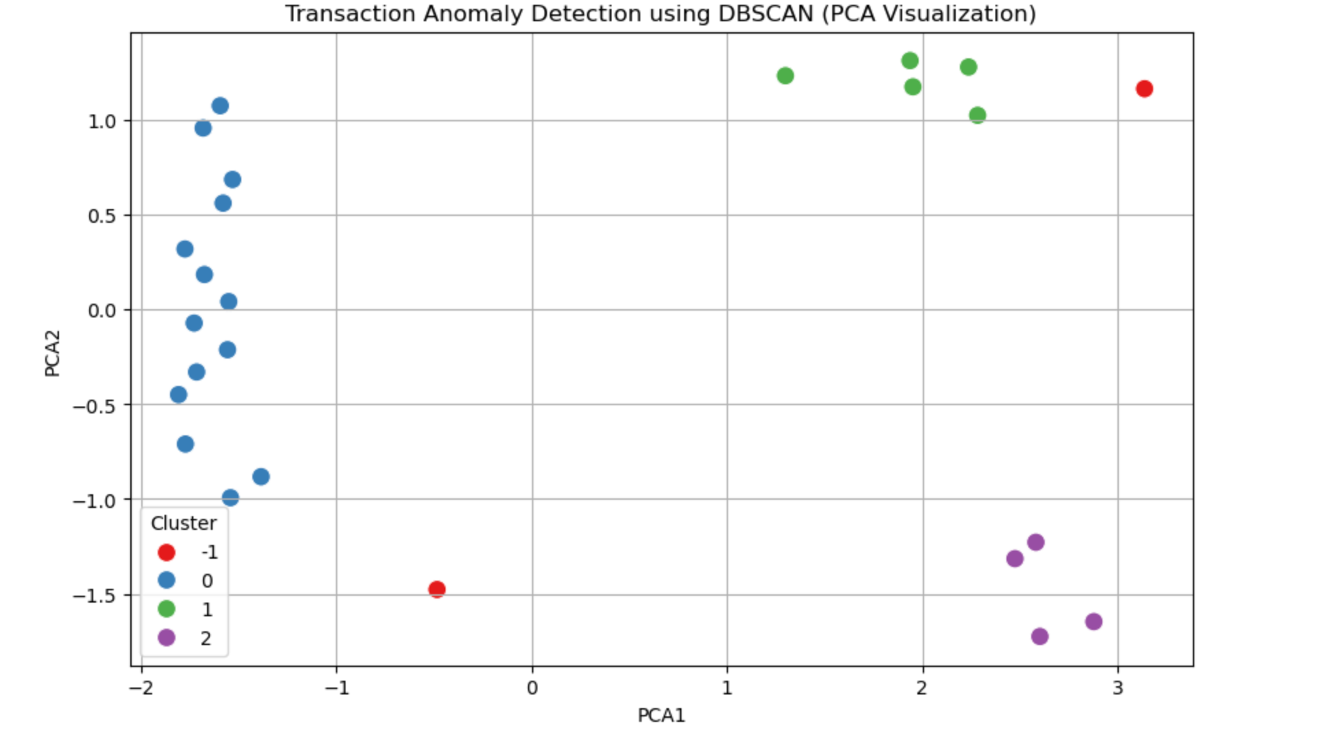
📈 What Does the DBSCAN Graph Show?
The PCA-based scatter plot visualizes how DBSCAN clustered the transactions:
- Cluster 0 and Cluster 1 are dense groups of similar transactions — most likely representing normal user behavior.
- Cluster 2 may represent a smaller group with distinct but still acceptable behavior.
- Any points labeled as -1 (not shown in this setup but often present) would be considered outliers or potential frauds.
🔍 DBSCAN has automatically:
- Grouped similar transactions based on their characteristics (amount, device score, fraud history, etc.)
- Flagged any abnormal or suspicious transactions as noise — making it easier for banks to investigate fraud.
💬 Join the DecodeAI WhatsApp Channel for regular AI updates → Click here