[Day 24] Unsupervised Machine Learning Type 7 – UMAP (with a Small Python Project)
UMAP turns messy customer or session data into crystal-clear 2D clusters—see normal users, bots & outliers like a pro! ⚡📊
![[Day 24] Unsupervised Machine Learning Type 7 – UMAP (with a Small Python Project)](https://storage.ghost.io/c/55/e8/55e827ca-bf8d-4eee-bdb4-ee48e49a011a/content/images/size/w2000/2025/03/UMAP.svg)
🎯 What is UMAP?
UMAP (Uniform Manifold Approximation and Projection) is a machine learning technique for dimensionality reduction, just like PCA or t-SNE — but smarter, faster, and more scalable.
While PCA focuses on preserving variance and t-SNE on local neighbors, UMAP captures both the global shape and local clusters in your data — and works like a charm on real-world, messy datasets.
Unlike PCA, which focuses on broad trends, or t-SNE, which hones in on local cliques, UMAP does both—it keeps nearby points tight while respecting the bigger picture.
Example: Say you’ve got employee performance data with metrics like hours worked, sales closed, emails sent, meetings attended, etc. That’s a multidimensional headache. UMAP can shrink it into a 2D scatterplot where each dot is an employee, and similar performers—like the sales superstars or the chronic procrastinators—cluster together. It’s about spotting the patterns that matter.
Let's take one more:
👨💻 Real-World Use Case: Cybersecurity Session Monitoring
Imagine you're a cybersecurity analyst. You’re monitoring user sessions on a high-traffic application, trying to:
- Detect bot activity
- Identify suspicious patterns
- Group normal users by behavior
Each session comes with user activity metrics, like time spent, clicks, scroll depth, and login patterns. That’s a high-dimensional dataset — hard to plot, harder to interpret.
UMAP lets you squish that data into 2D, revealing meaningful clusters of:
- 👨 Normal users
- 🤖 Bots
- ❗ Suspicious users
See the video belowa for better understanding
⚡ Why Use UMAP in This Case?
- ⚡ Scales fast for real-time behavioral data
- 🔍 Detects behavioral patterns without needing labels
- 🚫 Flags outliers like bots or potential attackers
- 📊 Helps visualize user segmentation for risk monitoring
Python Project : Customer Behavior Explorer
Imagine you’re a retail analyst with customer data from an online store. Each customer has features like total spend, items bought, browsing time, and return rate. You want to see how these customer groups—maybe to tailor marketing campaigns—but the data’s in a high-dimensional space (4+ variables), and you need it in 2D. Let’s analyze a small dataset of 25 customers to see how UMAP reveals shopping behavior patterns.
Each customer is described by 4 features:
- Total Spend: Dollars spent in the last year (e.g., $50 to $2000).
- Items Bought: Number of items purchased (e.g., 1 to 50).
- Browsing Time: Minutes spent on the site per visit (e.g., 5 to 60).
- Return Rate: Percentage of items returned (e.g., 0% to 50%).
This is a 4D dataset—each customer is a point in 4D space, too tricky to visualize directly. UMAP will map it to 2D for us.
Data Set: Save it as customers_list.csv
| Total Spend | Items Bought | Browsing Time | Return Rate | Customer Type |
|---|---|---|---|---|
| 150.0 | 5 | 10 | 0.10 | Casual |
| 120.0 | 3 | 8 | 0.05 | Casual |
| 180.0 | 6 | 12 | 0.15 | Casual |
| 140.0 | 4 | 9 | 0.08 | Casual |
| 160.0 | 5 | 11 | 0.12 | Casual |
| 1200.0 | 25 | 45 | 0.05 | Big Spender |
| 1500.0 | 30 | 50 | 0.03 | Big Spender |
| 1300.0 | 28 | 48 | 0.06 | Big Spender |
| 1100.0 | 22 | 40 | 0.04 | Big Spender |
| 1400.0 | 27 | 47 | 0.07 | Big Spender |
| 300.0 | 15 | 20 | 0.40 | Returner |
| 350.0 | 18 | 25 | 0.45 | Returner |
| 280.0 | 12 | 18 | 0.35 | Returner |
| 320.0 | 16 | 22 | 0.42 | Returner |
| 290.0 | 14 | 19 | 0.38 | Returner |
| 80.0 | 2 | 30 | 0.02 | Browser |
| 60.0 | 1 | 35 | 0.01 | Browser |
| 90.0 | 3 | 28 | 0.03 | Browser |
| 70.0 | 2 | 32 | 0.02 | Browser |
| 85.0 | 1 | 33 | 0.01 | Browser |
| 170.0 | 7 | 13 | 0.09 | Casual |
| 1250.0 | 26 | 46 | 0.05 | Big Spender |
| 310.0 | 17 | 21 | 0.39 | Returner |
| 75.0 | 2 | 31 | 0.02 | Browser |
| 145.0 | 5 | 10 | 0.11 | Casual |
✅ Python Code
?
# Import Libraries
import pandas as pd
import umap
import matplotlib.pyplot as plt
import seaborn as sns
from sklearn.preprocessing import StandardScaler
import warnings

# Suppress UMAP warning about n_jobs
warnings.filterwarnings("ignore", message="n_jobs value 1 overridden to 1 by setting random_state")

# Load the Dataset
df = pd.read_csv('customers_list.csv')

# Prepare Data for UMAP
X = df[['Total Spend', 'Items Bought', 'Browsing Time', 'Return Rate']]
y = df['Customer Type']

# Standardize the Features
scaler = StandardScaler()
X_scaled = scaler.fit_transform(X)

# Apply UMAP
umap_model = umap.UMAP(n_components=2, n_neighbors=5, random_state=42)
X_umap = umap_model.fit_transform(X_scaled)

# Create a DataFrame with UMAP Results
umap_df = pd.DataFrame(X_umap, columns=['UMAP1', 'UMAP2'])
umap_df['Customer Type'] = y

# Plot the Results
plt.figure(figsize=(10, 8))
sns.scatterplot(data=umap_df, x='UMAP1', y='UMAP2', hue='Customer Type', palette='deep', s=100, alpha=0.7)
plt.title('UMAP Visualization of 25 Customers Dataset')
plt.xlabel('UMAP Dimension 1')
plt.ylabel('UMAP Dimension 2')
plt.legend(title='Customer Type')
plt.grid(True)
plt.show()
Result:
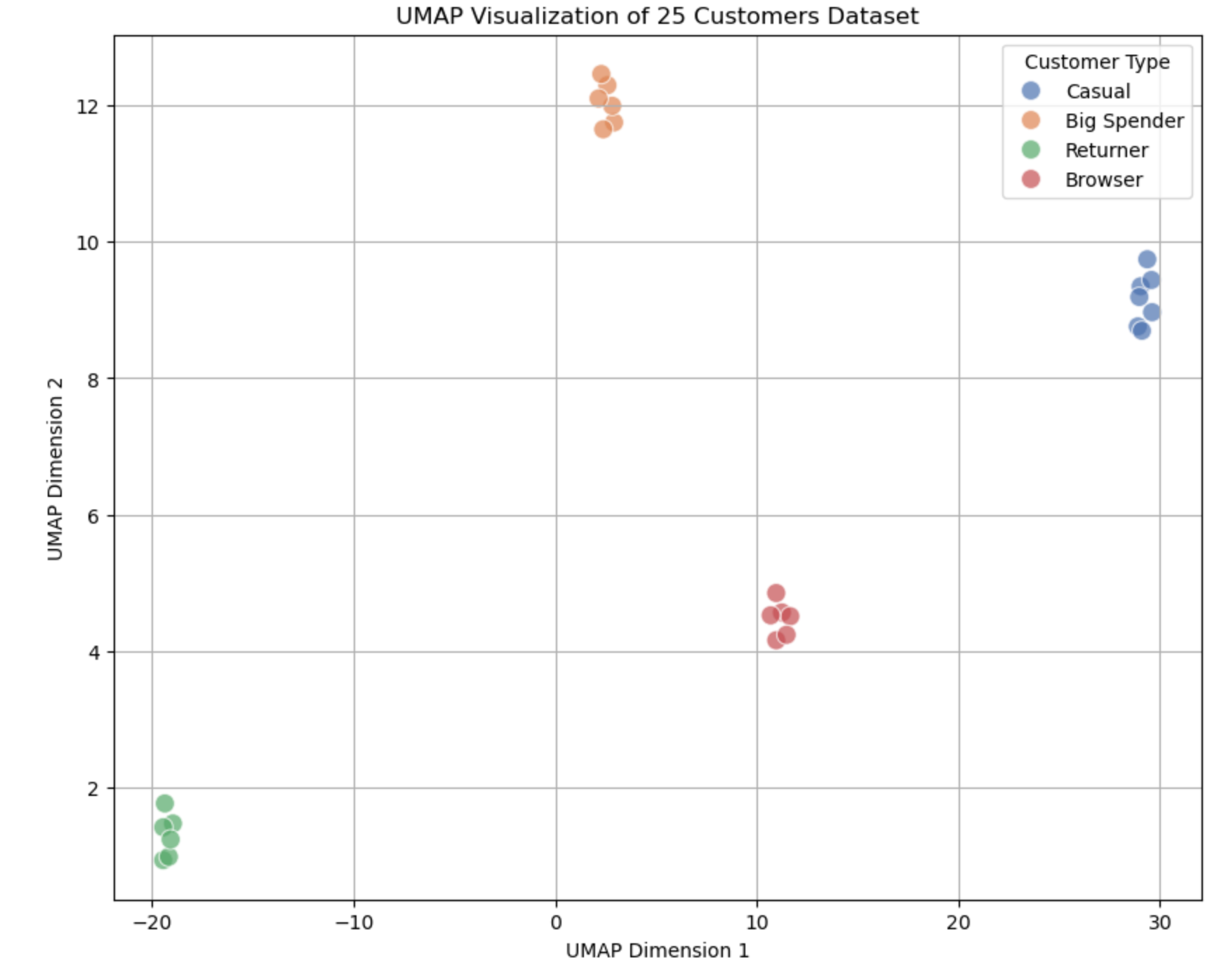
What the Output Graph Looks Like
Layout Explanation:
- Clusters: Expect 4 distinct groups:
- Casual: ~7 points (low spend ~$120–$180, few items, short browsing).
- Big Spender: ~6 points (high spend ~$1100–$1500, many items, long browsing).
- Returner: ~6 points (moderate spend ~$280–$350, high return rates).
- Browser: ~6 points (low spend ~$60–$90, long browsing, few items).
- Separation: Clusters should be clear, with UMAP keeping similar customers close and dissimilar ones apart, while preserving some global relationships (e.g., Casual might be nearer to Browser than Big Spender).
How about doing another project?
"BotRadar – Visualizing User Sessions to Detect Anomalies"
Dataset:
📋 Cybersecurity Session Dataset (25 Samples)
| Session Length | Pages Visited | Clicks | Scroll Depth (%) | Login Frequency | User Type |
|---|---|---|---|---|---|
| 512 | 14 | 22 | 88.30 | 2 | Normal |
| 767 | 9 | 47 | 41.88 | 9 | Normal |
| 853 | 1 | 44 | 10.87 | 7 | Normal |
| 84 | 10 | 8 | 28.33 | 4 | Normal |
| 143 | 9 | 24 | 86.40 | 3 | Normal |
| 650 | 12 | 11 | 58.34 | 1 | Bot |
| 415 | 2 | 16 | 20.36 | 3 | Bot |
| 828 | 6 | 35 | 31.62 | 8 | Bot |
| 912 | 3 | 39 | 95.36 | 9 | Bot |
| 320 | 16 | 5 | 35.60 | 5 | Bot |
| 172 | 7 | 25 | 54.53 | 8 | Suspicious |
| 58 | 15 | 40 | 39.67 | 1 | Suspicious |
| 85 | 17 | 35 | 41.26 | 3 | Suspicious |
| 697 | 19 | 34 | 46.69 | 8 | Suspicious |
| 900 | 2 | 33 | 13.44 | 5 | Suspicious |
| 520 | 17 | 26 | 82.82 | 9 | Normal |
| 927 | 6 | 11 | 88.99 | 3 | Normal |
| 720 | 10 | 8 | 45.04 | 5 | Bot |
| 341 | 6 | 13 | 28.55 | 7 | Bot |
| 184 | 13 | 6 | 34.33 | 4 | Suspicious |
| 743 | 5 | 34 | 31.04 | 8 | Normal |
| 878 | 8 | 43 | 73.40 | 5 | Bot |
| 177 | 15 | 12 | 42.66 | 2 | Suspicious |
| 521 | 7 | 40 | 37.97 | 7 | Normal |
| 363 | 4 | 41 | 98.36 | 6 | Bot |
✅ Python Code
# pip install umap-learn

import pandas as pd
import matplotlib.pyplot as plt
import seaborn as sns
import umap
from sklearn.preprocessing import StandardScaler

# Step 1: Load the dataset
df = pd.read_csv("cyber_user_behavior_umap.csv")
X = df.drop(columns=["User Type"])
y = df["User Type"]

# Step 2: Scale the features
scaler = StandardScaler()
X_scaled = scaler.fit_transform(X)

# Step 3: Apply UMAP
reducer = umap.UMAP(n_components=2, n_neighbors=4, min_dist=0.4, random_state=42)
X_umap = reducer.fit_transform(X_scaled)

# Step 4: Visualize the results
umap_df = pd.DataFrame(X_umap, columns=["UMAP1", "UMAP2"])
umap_df["User Type"] = y

plt.figure(figsize=(10, 8))
sns.scatterplot(data=umap_df, x="UMAP1", y="UMAP2", hue="User Type", palette="Set2", s=120)
plt.title("UMAP Projection of Cybersecurity User Sessions")
plt.grid(True)
plt.xlabel("UMAP Dimension 1")
plt.ylabel("UMAP Dimension 2")
plt.legend(title="User Type")
plt.show()
Result:
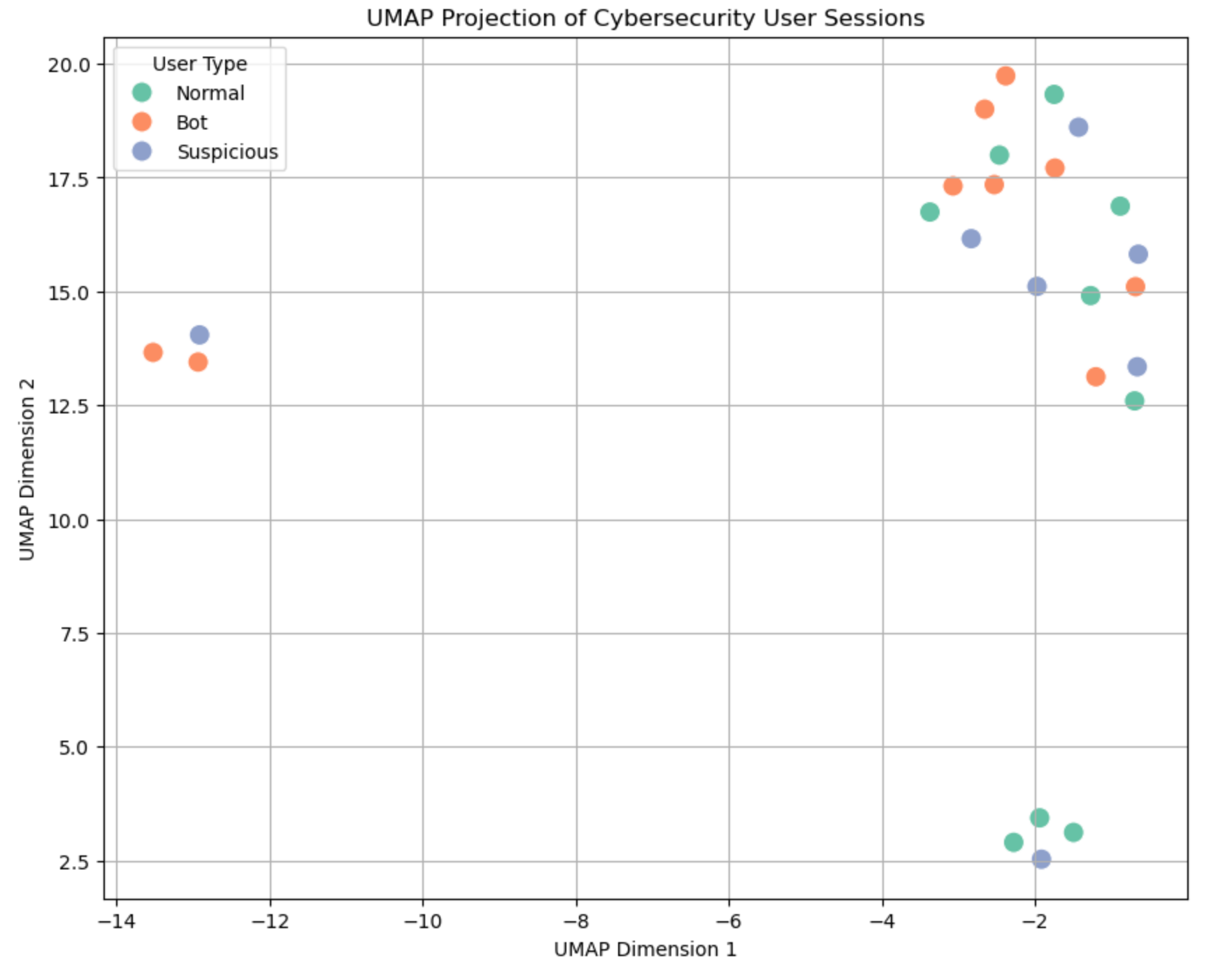
🧑💻 Color Legend: What the User Types Mean
- 🟢 Normal users: Typical browsing behavior — steady clicks, scrolls, and login patterns.
- 🟠 Bots: Often low scroll, few pages, repetitive or fast activity.
- 🔵 Suspicious: In-between behavior — might be real users doing weird things, or bots trying to mimic users.
💬 Join the DecodeAI WhatsApp Channel for regular AI updates → Click here