[Day 25] Unsupervised Machine Learning Type 8 – Gaussian Mixture Models (with a Practical Python Project)
Discover how Gaussian Mixture Models uncover hidden customer types like “Happy,” “Picky,” and “Grumbler”—with real-world nuance and clarity. 🎯📊
![[Day 25] Unsupervised Machine Learning Type 8 – Gaussian Mixture Models (with a Practical Python Project)](https://storage.ghost.io/c/55/e8/55e827ca-bf8d-4eee-bdb4-ee48e49a011a/content/images/size/w2000/2025/03/GMM.svg)
🎯 What is a Gaussian Mixture Model (GMM)?
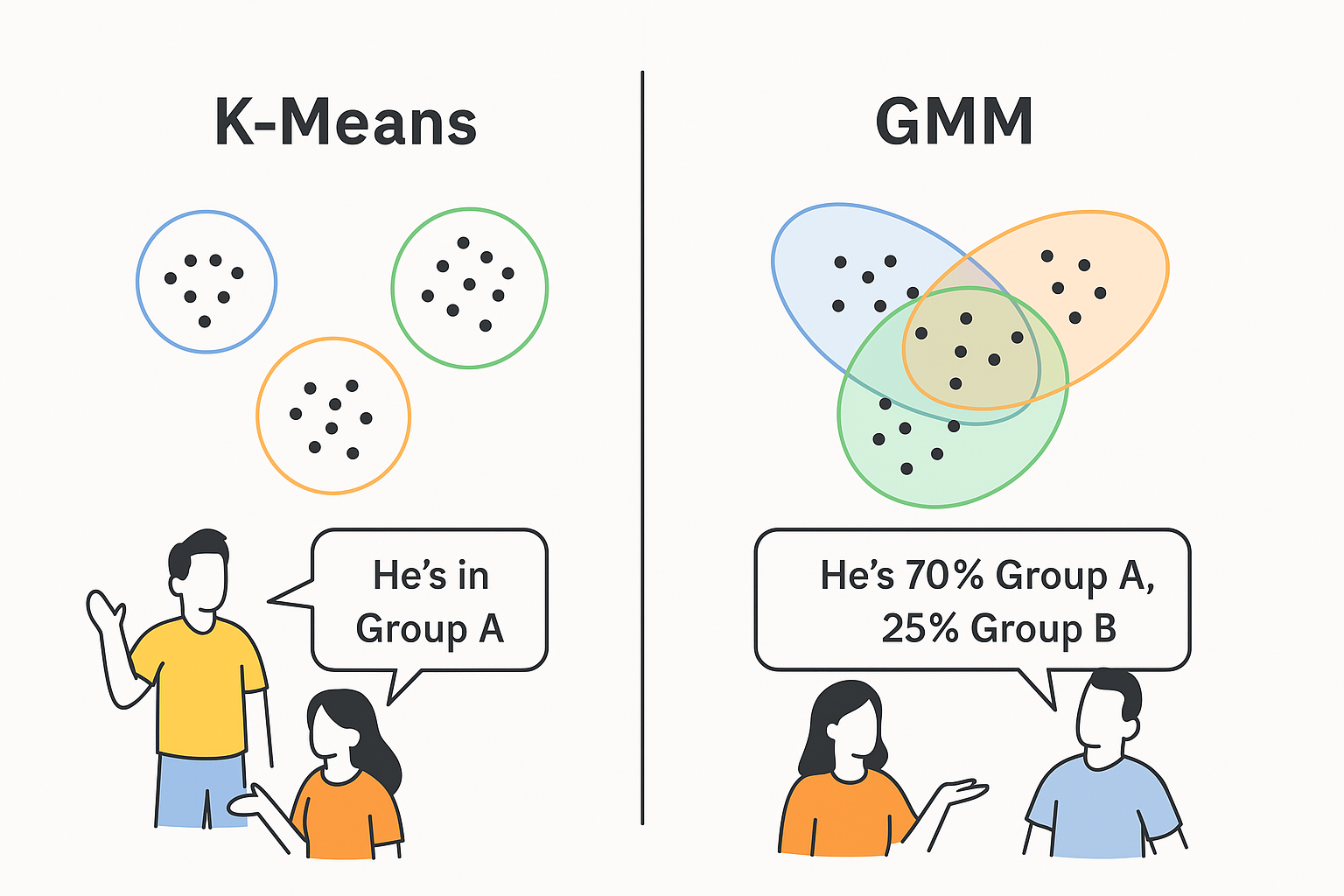
A Gaussian Mixture Model (GMM) is a smart tool in machine learning that imagines your data as a blend of different groups, each looking like a smooth, bell-shaped hill. It’s a hands-off method—it doesn’t need you to tell it what’s what. Instead, it checks out your data and thinks, “Hey, I see some overlapping bunches here—let’s sort them out!” It’s an unsupervised method, meaning it doesn’t need labels to figure things out.
Unlike k-means, which assumes hard, spherical clusters, GMM is softer and more flexible. It allows clusters to stretch, tilt, and overlap, assigning each data point a probability of belonging to multiple groups. Think of it as a chef tasting a stew and guessing how many ingredients went in—and how much of each.
Example: Imagine you’re analyzing student test scores across subjects like math, science, and reading. Some students are all-around stars, some struggle across the board, and others are mixed—great at math but weak in reading. That’s a multidimensional puzzle. GMM can sift through this data and identify these “types” of students, even if their scores overlap a bit. It’s about finding the hidden flavors in the mix.
👨💻 Real-World Use Case: Customer Satisfaction Analysis
Picture yourself as a product manager at a company like Amazon or Netflix. You’ve got survey data from users rating things like delivery speed, product quality, customer service, and ease of use. Your goal? Figure out:
- Who’s happy overall
- Who’s frustrated with specific things
- Who’s neutral but picky about one aspect
Each survey response has metrics like satisfaction scores (1–5) across multiple categories. That’s a high-dimensional dataset—tough to eyeball. GMM steps in to model this as a blend of “satisfaction groups”—say, “Super Fans,” “Complainers,” and “Meh”—without needing predefined labels. It’ll tell you not just who’s in each group, but how likely they are to fit there.
Why GMM Shines?
- Scales to messy data: Handles overlapping behaviors (e.g., a “happy” customer might still hate slow shipping).
- Finds soft clusters: Some users might be 70% “Super Fan,” 30% “Meh”—GMM captures that nuance.
- Spots hidden trends: Reveals satisfaction patterns you didn’t know existed.
- Guides action: Pinpoints who needs a discount, a follow-up, or a feature fix.
⚡ Why Use GMM? Real-World Style
- Unravel the Overlap: Got data where groups blend? GMM sorts it out without forcing hard boundaries.
- Guess the Mix: It’s great for figuring out “how many types” are in your data, like how many customer personas you’ve got.
- Catch the Subtle: Outliers or edge cases get flagged with low probabilities and are not ignored.
- Set Up Smart Moves: Use it to segment users, products, or behaviors for targeted strategies.
⚡ Why GMM Rocks in the Real World
- Digs Up Stories: Tracking fitness app users? GMM might find clusters of “casual walkers,” “gym rats,” and “weekend warriors” based on steps, workouts, and app time—insights you’d miss in averages.
- Explains the Gray Areas: Your sales team sees “hot leads” vs. “cold leads.” GMM plots a spectrum—some leads are 60% hot, 40% cold—helping you prioritize.
- Fixes Sneaky Issues: Analyzing machine sensor data? GMM could spot “normal,” “kinda failing,” and “about to break” clusters before disaster hits.
- Everyday Examples:
- Healthcare: Grouping patients by symptoms and vitals to spot disease stages (e.g., mild vs. severe diabetes).
- Marketing: Segmenting email subscribers by open rates and clicks for personalized campaigns.
- Finance: Modeling stock trading behaviors to detect normal vs. erratic patterns.
Python Project: Customer Satisfaction Classifier
Imagine you’re a product analyst with survey data from 25 customers who rated your online store on four aspects: delivery speed, product quality, customer service, and website ease. You want to group them into satisfaction types—like “Happy Campers,” “Picky Critics,” or “Grumblers”—to tweak your strategy. The data’s in 4D space (four features), and GMM will help us uncover these groups.
Each customer is described by 4 features (scores from 1–5):
- Delivery Speed: How fast they got their stuff (1 = slow, 5 = lightning).
- Product Quality: How they liked the goods (1 = junk, 5 = awesome).
- Customer Service: How they rated support (1 = rude, 5 = stellar).
- Website Ease: How easy the site was to use (1 = maze, 5 = breeze).
This is a 4D dataset—too complex to visualize directly. GMM will model it as a mix of clusters and give us probabilities for each customer’s group.
Data Set: Save it as customer_satisfaction.csv
| Delivery Speed | Product Quality | Customer Service | Website Ease | Satisfaction Type |
|---|---|---|---|---|
| 4.2 | 4.5 | 4.8 | 4.0 | Happy |
| 4.0 | 4.7 | 4.5 | 4.3 | Happy |
| 4.5 | 4.2 | 4.6 | 4.1 | Happy |
| 4.1 | 4.8 | 4.7 | 4.2 | Happy |
| 4.3 | 4.4 | 4.9 | 4.5 | Happy |
| 2.0 | 3.5 | 2.8 | 3.0 | Picky |
| 2.5 | 3.8 | 3.0 | 2.7 | Picky |
| 1.8 | 3.2 | 2.5 | 3.1 | Picky |
| 2.2 | 3.6 | 2.9 | 2.8 | Picky |
| 2.3 | 3.4 | 2.7 | 3.3 | Picky |
| 1.5 | 1.8 | 2.0 | 1.7 | Grumbler |
| 1.7 | 2.0 | 1.9 | 1.5 | Grumbler |
| 1.3 | 1.6 | 2.1 | 1.8 | Grumbler |
| 1.9 | 2.2 | 1.8 | 1.6 | Grumbler |
| 1.4 | 1.7 | 2.3 | 1.9 | Grumbler |
| 4.6 | 4.1 | 4.4 | 4.7 | Happy |
| 2.1 | 3.9 | 2.6 | 2.9 | Picky |
| 1.6 | 1.9 | 2.2 | 1.4 | Grumbler |
| 4.4 | 4.6 | 4.3 | 4.8 | Happy |
| 2.4 | 3.3 | 2.4 | 3.2 | Picky |
| 1.8 | 2.1 | 1.7 | 2.0 | Grumbler |
| 4.7 | 4.3 | 4.5 | 4.6 | Happy |
| 2.6 | 3.7 | 3.1 | 2.5 | Picky |
| 1.5 | 1.5 | 1.6 | 1.8 | Grumbler |
| 4.0 | 4.9 | 4.8 | 4.4 | Happy |
✅ Python Code
Install Dependencies:
pip install pandas numpy scikit-learn matplotlib seaborn
# Import Libraries
import pandas as pd
import numpy as np
from sklearn.mixture import GaussianMixture
import matplotlib.pyplot as plt
import seaborn as sns
from sklearn.preprocessing import StandardScaler

# Load the Dataset
df = pd.read_csv('customer_satisfaction.csv')


# Prepare Data for GMM
X = df[['Delivery Speed', 'Product Quality', 'Customer Service', 'Website Ease']]
y_true = df['Satisfaction Type']  # For comparison, not used in GMM fitting

# Standardize the Features
scaler = StandardScaler()
X_scaled = scaler.fit_transform(X)

# Apply GMM
gmm = GaussianMixture(n_components=3, random_state=42)  # 3 clusters: Happy, Picky, Grumbler
gmm.fit(X_scaled)
labels = gmm.predict(X_scaled)
probs = gmm.predict_proba(X_scaled)  # Probability of belonging to each cluster

# Add GMM Results to DataFrame
gmm_df = pd.DataFrame(X_scaled, columns=['Delivery Speed', 'Product Quality', 'Customer Service', 'Website Ease'])
gmm_df['Cluster'] = labels
gmm_df['True Type'] = y_true

# For Visualization, Reduce to 2D with PCA (GMM doesn’t give 2D directly)
from sklearn.decomposition import PCA
pca = PCA(n_components=2)
X_pca = pca.fit_transform(X_scaled)
pca_df = pd.DataFrame(X_pca, columns=['PC1', 'PC2'])
pca_df['Cluster'] = labels
pca_df['True Type'] = y_true

# Plot the Results
plt.figure(figsize=(10, 8))
sns.scatterplot(data=pca_df, x='PC1', y='PC2', hue='Cluster', style='True Type', palette='deep', s=100, alpha=0.7)
plt.title('GMM Clustering of 25 Customers (Visualized with PCA)')
plt.xlabel('Principal Component 1')
plt.ylabel('Principal Component 2')
plt.legend(title='Cluster / True Type')
plt.grid(True)
plt.show()
Result: What the Output Looks Like
When you run this, you’ll get two key outputs:
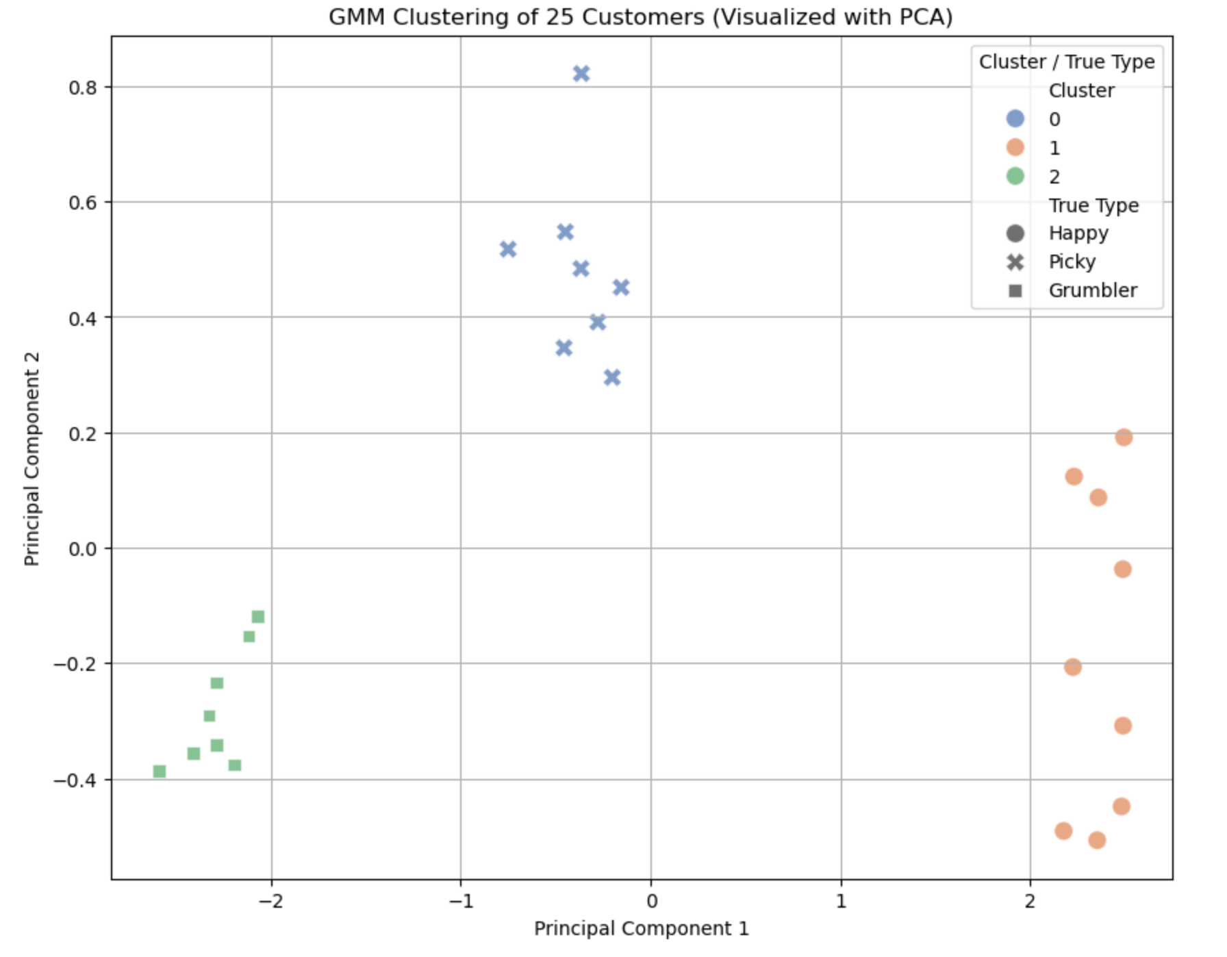
Axes:
- X-axis: “Principal Component 1” (PC1).
- Y-axis: “Principal Component 2” (PC2).
These are simplified dimensions from the 4D data.
Layout Explanation:
- Clusters: Expect 3 distinct groups:
- Happy: ~9 points (high scores ~4–5 across all features).
- Picky: ~8 points (mixed scores, e.g., low delivery ~2, higher quality ~3.5).
- Grumbler: ~8 points (low scores ~1.5–2 across the board).
Summary of the Output
- What We See: Three clusters representing satisfaction types (Happy, Picky, Grumbler), visualized in 2D via PCA, with probabilities showing how “sure” GMM is about each customer.
- Useful Results:
- Confirms distinct satisfaction groups: Happy customers love everything, Picky ones nitpick (e.g., hate slow delivery), Grumblers dislike most aspects.
- Probabilities reveal nuance—e.g., a customer might be 60% Picky, 40% Grumbler, hinting at mixed feelings.
- Practical Use:
- Targeted Fixes: Send faster shipping offers to Picky customers, apologies to Grumblers, and perks to Happy ones.
- Customer Insights: Understand satisfaction drivers—e.g., low delivery scores drag some into Picky territory.
- Strategy Planning: Prioritize improvements (e.g., website ease) based on cluster sizes and complaints.
and yes, that's it.
💬 Join the DecodeAI WhatsApp Channel for regular AI updates → Click here