[Day 26] Unsupervised Machine Learning Type 9 – Autoencoders (with a Practical Python Project)
Meet Autoencoders: the unsupervised neural nets that learn what “normal” looks like—then flag what isn’t. Think fraud, glitches, or patterns gone weird.
![[Day 26] Unsupervised Machine Learning Type 9 – Autoencoders (with a Practical Python Project)](https://storage.ghost.io/c/55/e8/55e827ca-bf8d-4eee-bdb4-ee48e49a011a/content/images/size/w2000/2025/03/AE.svg)
🎯 What is an Autoencoder?
An Autoencoder is a nifty machine learning trick that acts like a super-smart photocopier. It takes a big, messy pile of data, squeezes it down to a tiny “summary” version, and then tries to rebuild the original from that summary—all without being told what’s important. It’s unsupervised, meaning it , , like a kid figuring out how to pack a suitcase by trial and error.
Imagine you’re at a crowded party with lots of chatter, music, laughter, and clinking glasses. An Autoencoder is like your brain tuning out the noise to catch just the key conversations, then later retelling them with most of the details intact. It finds the “essence” of your data by compressing it (encoding) and then uncompressing it (decoding), learning what matters most along the way.
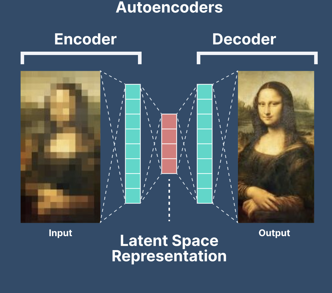
Example: Picture a stack of blurry pet photos—dogs, cats, maybe a sneaky hamster. An Autoencoder could squish each photo into a smaller “code” (like a sketch), then recreate the images from that code. Even if some fur gets fuzzy, it learns what makes a dog a dog or a cat a cat. It’s about boiling down the chaos into something simple, then bringing it back to life.
How does it work?

See video below for a better understanding:
👨💻 Real-World Use Case: Credit Card Fraud Detection
Imagine you’re a fraud analyst at a bank. You’ve got millions of credit card transactions rolling in—amounts, locations, times, merchant types. Most are legit, but a few are sneaky fraudsters. Your mission? Spot the weird ones fast. Each transaction is a jumble of numbers, too complex to sift through manually.
An Autoencoder steps in like a security guard with a superpower. It learns what “normal” transactions look like by compressing and rebuilding them—say, $50 at a coffee shop, $200 at a grocery store. When a weird one pops up—like $5,000 in a foreign casino at 3 a.m.—it struggles to rebuild it, because it doesn’t fit the pattern. That “rebuild error” flags it as suspicious.
Why Autoencoders Shine Here:
- Spots the oddballs: Big errors mean something’s off—no fraud labels needed.
- Handles tons of data: Scales to millions of transactions without breaking a sweat.
- Learns on the fly: Adapts to new “normal” patterns as spending habits shift.
- Saves the day: Alerts you to investigate fishy activity before it’s too late.
⚡ Why Use Autoencoders? Real-World Style
- Shrink the Noise: Got messy, high-dimensional data? Autoencoders cut through the clutter to find what counts.
- Spot the Strange: They’re ace at flagging stuff that doesn’t fit—like a glitch or a fraudster.
- Simplify the Complex: Turn a data jungle into a neat little map you can actually use.
- Boost Other Tools: Use that “summary” code for clustering, visualization, or feeding into other models.
⚡ Why Autoencoders Rock in the Real World
- Unmasks Hidden Gems: Monitoring factory machines? Autoencoders can compress sensor readings and flag odd vibrations, catching breakdowns before they happen.
- Cuts Through the Fog: Got grainy security footage? They can clean it up by learning what a “normal” scene looks like, making faces or plates clearer.
- Sniffs Out Trouble: Tracking website clicks? Autoencoders spot bot traffic—clicks that don’t rebuild like human patterns.
- Everyday Examples:
- Healthcare: Compressing patient scans to detect anomalies like tumors.
- Retail: Shrinking customer profiles to find unusual buying spikes.
- Music: Denoising old recordings by learning clean sound patterns.
Python Project: Transaction Anomaly Finder
Imagine you’re a bank analyst with data from 25 credit card transactions. Each has features like amount, time of day, merchant category, and distance from home. You want to spot weird transactions—like fraud or errors—without labeling them first. The data’s in 4D space (four features), and an Autoencoder will learn the “normal” pattern and flag outliers.
Each transaction is described by 4 features:
- Amount: Dollars spent ($5–$1000).
- Time of Day: Hour in 24-hour format (0–23).
- Merchant Category: Code for store type (1–5, e.g., 1 = grocery, 5 = luxury).
- Distance: Miles from home (0–100).
This is a 4D dataset—too tricky to eyeball. The Autoencoder will compress it to a 2D “code,” rebuild it, and highlight transactions that don’t fit.
Data Set: Save it as transactions_data.csv
| Amount | Time of Day | Merchant Category | Distance | Transaction Type |
|---|---|---|---|---|
| 50.0 | 9 | 1 | 2.0 | Normal |
| 75.0 | 12 | 1 | 3.5 | Normal |
| 30.0 | 8 | 2 | 1.8 | Normal |
| 120.0 | 14 | 1 | 4.0 | Normal |
| 60.0 | 10 | 3 | 2.5 | Normal |
| 800.0 | 3 | 5 | 75.0 | Fraud |
| 950.0 | 2 | 5 | 90.0 | Fraud |
| 700.0 | 4 | 4 | 60.0 | Fraud |
| 850.0 | 1 | 5 | 85.0 | Fraud |
| 600.0 | 5 | 4 | 70.0 | Fraud |
| 45.0 | 11 | 2 | 3.0 | Normal |
| 90.0 | 13 | 1 | 2.8 | Normal |
| 25.0 | 7 | 3 | 1.5 | Normal |
| 110.0 | 15 | 1 | 4.5 | Normal |
| 70.0 | 9 | 2 | 2.2 | Normal |
| 500.0 | 23 | 5 | 50.0 | Fraud |
| 55.0 | 10 | 1 | 3.2 | Normal |
| 880.0 | 0 | 4 | 95.0 | Fraud |
| 40.0 | 8 | 2 | 1.9 | Normal |
| 130.0 | 16 | 1 | 4.8 | Normal |
| 650.0 | 6 | 5 | 65.0 | Fraud |
| 80.0 | 12 | 3 | 2.7 | Normal |
| 35.0 | 9 | 1 | 2.0 | Normal |
| 720.0 | 4 | 4 | 80.0 | Fraud |
| 100.0 | 11 | 2 | 3.8 | Normal |
✅ Python Code
Install Dependencies:
pip install pandas numpy scikit-learn tensorflow matplotlib seaborn
# Import Libraries
import pandas as pd
import numpy as np
from sklearn.preprocessing import StandardScaler
import tensorflow as tf
from tensorflow.keras import layers, models
import matplotlib.pyplot as plt
import seaborn as sns

# Load the Dataset
df = pd.read_csv('transactions_data.csv')
print("Dataset loaded:")
print(df.head())

# Prepare Data for Autoencoder
X = df[['Amount', 'Time of Day', 'Merchant Category', 'Distance']]
y_true = df['Transaction Type']  # For comparison, not used in training

# Standardize the Features
scaler = StandardScaler()
X_scaled = scaler.fit_transform(X)

# Build the Autoencoder
input_dim = X_scaled.shape[1]  # 4 features
encoding_dim = 2  # Compress to 2D

# Encoder
autoencoder = models.Sequential([
    layers.Input(shape=(input_dim,)),
    layers.Dense(3, activation='relu'),
    layers.Dense(encoding_dim, activation='relu'),  # Bottleneck
    layers.Dense(3, activation='relu'),
    layers.Dense(input_dim, activation='linear')   # Decoder output
])

# Compile and Train
autoencoder.compile(optimizer='adam', loss='mse')
autoencoder.fit(X_scaled, X_scaled, epochs=50, batch_size=8, verbose=0)

# Get Reconstruction Errors
reconstructions = autoencoder.predict(X_scaled)
mse = np.mean(np.square(X_scaled - reconstructions), axis=1)  # Mean Squared Error per sample

# Add Results to DataFrame
result_df = pd.DataFrame(X_scaled, columns=['Amount', 'Time of Day', 'Merchant Category', 'Distance'])
result_df['MSE'] = mse
result_df['True Type'] = y_true

# Visualize with 2D PCA (for plotting)
from sklearn.decomposition import PCA
pca = PCA(n_components=2)
X_pca = pca.fit_transform(X_scaled)
pca_df = pd.DataFrame(X_pca, columns=['PC1', 'PC2'])
pca_df['MSE'] = mse
pca_df['True Type'] = y_true

# Plot the Results
plt.figure(figsize=(10, 8))
sns.scatterplot(data=pca_df, x='PC1', y='PC2', hue='True Type', size='MSE', palette='deep', alpha=0.7)
plt.title('Autoencoder Anomaly Detection in 25 Transactions (Visualized with PCA)')
plt.xlabel('Principal Component 1')
plt.ylabel('Principal Component 2')
plt.legend(title='Transaction Type')
plt.grid(True)
plt.show()

# Flag Anomalies (e.g., top 25% MSE)
threshold = np.percentile(mse, 75)
print(f"\nAnomaly Threshold (75th percentile MSE): {threshold:.4f}")
print("Transactions with MSE above threshold (potential anomalies):")
print(result_df[result_df['MSE'] > threshold][['MSE', 'True Type']])
Result: What the Output Looks Like
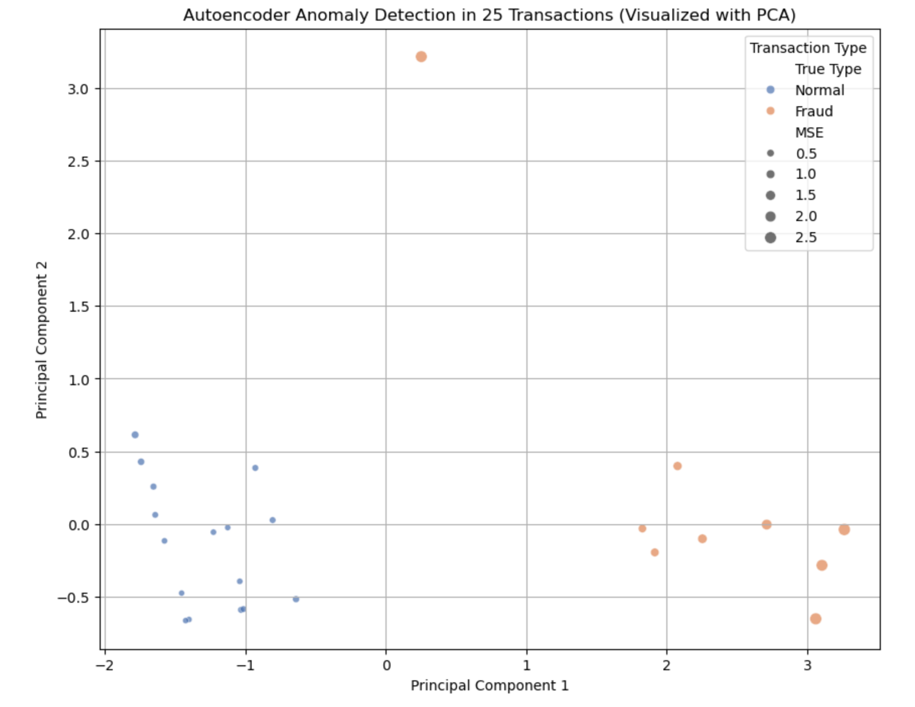
- Points: 25 dots, each a transaction.
- Pattern:
- Normal: ~16 points (small amounts ~$25–$130, daytime, low distance) cluster with small dots (low MSE).
- Fraud: ~9 points (big amounts ~$500–$950, odd hours, far distances) spread out with bigger dots (high MSE).
- Pattern:
Color Legend:
- Blue: Normal (tight cluster, small dots).
- Red: Fraud (scattered, larger dots)—the Autoencoder struggles to rebuild these, signaling anomalies.
Why is this useful here?
- What We See: Normal transactions cluster tightly with low error, while Fraud ones stand out with high error.
- Useful Results:
- Spots fraud without labels—high MSE flags big, odd-hour, far-away spends.
- Shows “how weird” each transaction is with MSE scores.
- Practical Use:
- Fraud Alerts: Investigate transactions above the threshold (e.g., $800 at 3 a.m., 75 miles away).
- Pattern Learning: Understand what “normal” looks like for better rules.
- Scalability: Ready for millions of transactions with the same logic.
This Autoencoder is your fraud-fighting sidekick—simple to grasp and sharp at catching the unusual.
BONUS:
Unsupervised Learning Algorithms Comparison
📊 Unsupervised Learning Algorithms Comparison
| Algorithm | Type | How It Works | Best Used When | Modern Use Cases |
|---|---|---|---|---|
| K-Means | Clustering | Partitions data into K clusters using centroids and minimizes within-cluster variance. | You know the number of clusters and want fast, simple segmentation. | Customer segmentation, image compression, document clustering. |
| Hierarchical Clustering | Clustering | Builds a hierarchy/tree of clusters based on distance/similarity. | You want interpretable dendrograms or don't know cluster count. | Social network analysis, gene expression studies, taxonomies. |
| DBSCAN | Clustering | Groups dense regions and identifies outliers as noise. | You expect irregularly shaped clusters or noise/outliers. | Fraud detection, anomaly spotting, spatial/geolocation clustering. |
| PCA | Dimensionality Reduction | Projects data onto orthogonal components that capture maximum variance. | You need a quick, linear reduction to visualize or prep for ML. | Preprocessing for ML models, face recognition, finance analytics. |
| ICA | Dimensionality Reduction | Separates independent sources from mixed signals using statistical independence. | You need to extract independent signals (e.g., audio separation). | Signal processing, neuroscience, audio source separation. |
| t-SNE | Dimensionality Reduction | Preserves local structure while reducing dimensions; non-linear. | You want to visualize high-dimensional data in 2D/3D, keeping local relationships. | Visualizing NLP embeddings, image feature exploration. |
| UMAP | Dimensionality Reduction | Preserves both local and global structures; graph-based and non-linear. | You want visualization with scalability, preserving both local/global relationships. | Large-scale embedding visualization, recommender systems. |
| Gaussian Mixture Models | Clustering | Assumes data is generated from multiple Gaussian distributions. | You need soft clustering (probabilities), better with overlapping clusters. | Market segmentation, speech modeling, probabilistic clustering. |
| Encoders (Autoencoders) | Dimensionality Reduction | Neural networks compress and reconstruct input, learning compact features. | You want to learn compressed representations (e.g., for anomaly detection or denoising). | Anomaly detection, feature learning, recommender systems, generative models. |
When to Use Which Algorithm?
- Clustering:
- Use K-Means for large, numeric datasets with clear spherical clusters.
- Use Hierarchical Clustering for small datasets needing interpretable hierarchies.
- Use DBSCAN for noisy data with irregular cluster shapes.
- Use GMM for probabilistic clustering (e.g., overlapping groups).
- Dimensionality Reduction:
- Use PCA for linear, high-variance feature extraction.
- Use ICA for separating mixed signals (e.g., audio).
- Use t-SNE/UMAP for visualizing high-dimensional data (t-SNE for local, UMAP for global+local).
- Use Autoencoders for non-linear, deep learning-based compression.
- Modern Trends:
- UMAP is replacing t-SNE for faster, scalable visualization.
- GMMs and VAEs (Variational Autoencoders) are popular in generative AI.
- DBSCAN is widely used in IoT/geospatial analytics.
Yeah.. That's it.
💬 Join the DecodeAI WhatsApp Channel for regular AI updates → Click here