[Day 29] Reinforcement Learning Type 2 – SARSA (with a Practical Python Project)

🎯 What is SARSA?

SARSA (State-Action-Reward-State-Action) is a savvy reinforcement learning method that teaches a machine to make smart moves by learning from its own steps, like a cautious hiker picking a trail. It stands for State-Action-Reward-State-Action, meaning it updates its strategy based on what it does now, what it gets, and what it plans to do next—all in one smooth loop. Unlike Q-Learning, which dreams big by always chasing the best possible future, SARSA sticks to reality, learning from the path it actually takes.

Picture a puppy learning to fetch a ball in a park. It tries a step—say, darting right—gets a pat (+reward) or a tumble (-reward), then picks its next move based on that experience. SARSA is like the puppy’s memory, noting: “Right at the tree got me a pat, so I’ll try right again next time I’m here.” It builds a guidebook (SARSA table) step-by-step, balancing bold tries with safe bets.

Example: Imagine a robot bartender mixing drinks. It picks an action—add ice—sees if the customer smiles (+reward) or frowns (-reward), then decides its next move (stir or pour) based on that. SARSA helps it learn a smooth routine by sticking to what it’s actually doing, not just the dreamiest outcome.

👨‍💻 Real-World Use Case: Smart Traffic Light Control

Imagine you’re a city planner tweaking traffic lights to ease rush-hour jams. Each intersection has states (car queues) and actions (green north-south or east-west). The goal? Minimize wait times (reward = fewer cars waiting). Sensors track queues, and lights switch every few seconds.

SARSA steps in like a traffic cop with a notebook. It tries “green north-south” at a busy corner, sees the queue shrink (+reward), then picks “green east-west” next, updating its plan based on what it just did—not the best possible switch it could’ve dreamed up. Over time, it learns a rhythm: “At 5 p.m., north-south first, then east-west clears the jam.”

Why SARSA Shines Here:

• Stays practical: Learns from real sequences, not hypothetical bests—fits messy traffic patterns.
• Adapts live: Adjusts as car flows shift, no pre-set rules needed.
• Smooths flow: Balances exploration (new timings) with exploitation (known good switches).
• Scales: Works across a grid of lights with consistent logic.

⚡ Why Use SARSA? Real-World Style

• Learn on the Go: No need for a perfect plan—SARSA figures it out from actual tries.
• Play It Safe: Updates based on real next steps, not risky “what ifs”—great for cautious tasks.
• Build Experience: Turns every move into a lesson, stacking up a solid strategy.
• Fit the Flow: Perfect for jobs where actions chain together, like routines or sequences.

⚡ Why SARSA Rocks in the Real World

• Guides the Careful: Training a drone to survey crops? SARSA learns: “Hover low here, then swing right”—sticking to what it’s doing, avoiding crashes.
• Tunes the Routine: Managing a robotic arm on an assembly line? It masters “grab, twist, place” by refining each step as it goes.
• Handles the Flux: Adjusting room temps in a smart home? SARSA tweaks “heat up, then fan” based on real weather shifts.
• Everyday Examples:
  • Healthcare: Teaching a rehab robot to adjust pressure—steady gains, no wild swings.
  • Gaming: Training an NPC to dodge traps—learns from its own moves, not just the optimal play.
  • Retail: Setting a chatbot’s replies—sticks to what’s working, improves chat by chat.

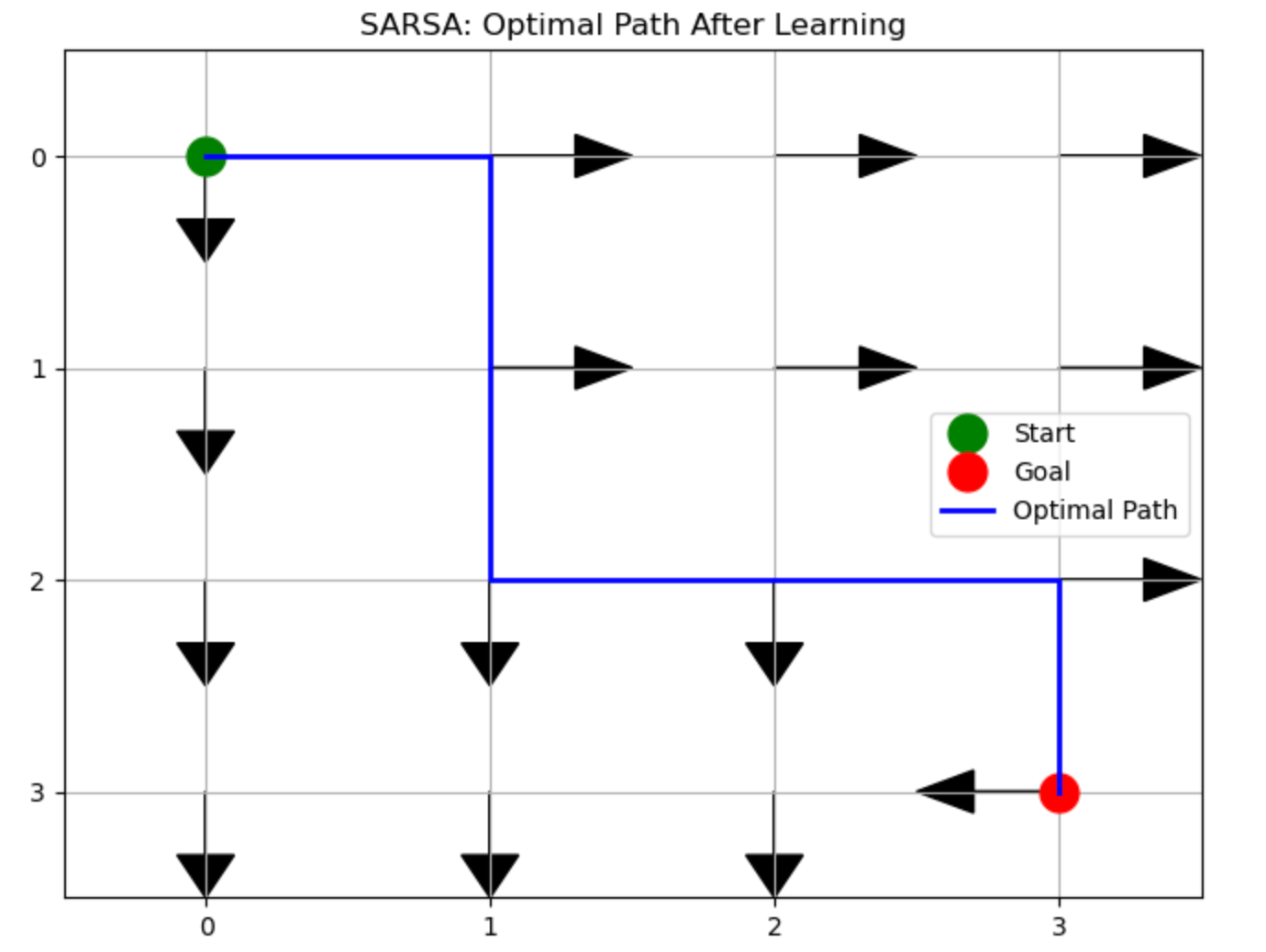
🛰 Project Name: SARSA Grid World Navigation

Goal: To demonstrate how the SARSA reinforcement learning algorithm learns to find the optimal path from a starting point to a goal in a simple grid environment. The agent learns through trial and error, receiving negative rewards for each step taken and a positive reward upon reaching the goal. The visualization shows how the agent gradually discovers the shortest path while avoiding unnecessary movements.

🐍 Python Code: SARSA Drone Navigation

import numpy as np
import matplotlib.pyplot as plt
import seaborn as sns

# Simple 4x4 grid world
class GridWorld:
    def __init__(self):
        self.rows, self.cols = 4, 4
        self.start = (0, 0)
        self.goal = (3, 3)
        self.state = self.start
        
        # Actions: up, right, down, left
        self.actions = [(-1, 0), (0, 1), (1, 0), (0, -1)]
        
    def reset(self):
        self.state = self.start
        return self.state
    
    def step(self, action_idx):
        # Move according to action
        action = self.actions[action_idx]
        row, col = self.state
        new_row = max(0, min(self.rows-1, row + action[0]))
        new_col = max(0, min(self.cols-1, col + action[1]))
        self.state = (new_row, new_col)
        
        # Reward: -1 per step, +10 at goal
        if self.state == self.goal:
            return self.state, 10, True
        else:
            return self.state, -1, False

# SARSA algorithm implementation
def sarsa(env, episodes=100, alpha=0.1, gamma=0.9, epsilon=0.1):
    # Initialize Q-table
    q_table = np.zeros((env.rows, env.cols, len(env.actions)))
    
    # For visualization
    rewards_history = []
    
    for episode in range(episodes):
        state = env.reset()
        row, col = state
        
        # Choose action using epsilon-greedy
        if np.random.random() < epsilon:
            action = np.random.randint(0, len(env.actions))
        else:
            action = np.argmax(q_table[row, col])
        
        total_reward = 0
        done = False
        
        while not done:
            # Take action, observe next state and reward
            next_state, reward, done = env.step(action)
            next_row, next_col = next_state
            total_reward += reward
            
            # Choose next action using epsilon-greedy
            if np.random.random() < epsilon:
                next_action = np.random.randint(0, len(env.actions))
            else:
                next_action = np.argmax(q_table[next_row, next_col])
            
            # SARSA update rule
            q_table[row, col, action] += alpha * (
                reward + gamma * q_table[next_row, next_col, next_action] - 
                q_table[row, col, action]
            )
            
            # Transition to next state and action
            row, col = next_row, next_col
            action = next_action
        
        rewards_history.append(total_reward)
        
        # Reduce exploration over time
        epsilon = max(0.01, epsilon * 0.95)
    
    return q_table, rewards_history

# Visualize path after learning
def visualize_path(env, q_table):
    # Get optimal policy
    policy = np.zeros((env.rows, env.cols), dtype=int)
    for r in range(env.rows):
        for c in range(env.cols):
            policy[r, c] = np.argmax(q_table[r, c])
    
    # Create the path visualization
    plt.figure(figsize=(8, 6))
    
    # Create grid
    plt.grid(True)
    plt.xlim(-0.5, env.cols-0.5)
    plt.ylim(-0.5, env.rows-0.5)
    plt.xticks(range(env.cols))
    plt.yticks(range(env.rows))
    
    # Flip y-axis to match grid coordinates
    plt.gca().invert_yaxis()
    
    # Plot start and goal
    plt.plot(env.start[1], env.start[0], 'go', markersize=15, label='Start')
    plt.plot(env.goal[1], env.goal[0], 'ro', markersize=15, label='Goal')
    
    # Plot optimal path
    state = env.start
    path = [state]
    while state != env.goal:
        r, c = state
        action = policy[r, c]
        dr, dc = env.actions[action]
        new_r = max(0, min(env.rows-1, r + dr))
        new_c = max(0, min(env.cols-1, c + dc))
        state = (new_r, new_c)
        path.append(state)
    
    # Convert path to x,y coordinates for plotting
    path_x = [p[1] for p in path]
    path_y = [p[0] for p in path]
    plt.plot(path_x, path_y, 'b-', linewidth=2, label='Optimal Path')
    
    # Add policy arrows
    for r in range(env.rows):
        for c in range(env.cols):
            action = policy[r, c]
            dx, dy = env.actions[action]
            plt.arrow(c, r, dx*0.3, dy*0.3, head_width=0.2, head_length=0.2, fc='k', ec='k')
    
    plt.title('SARSA: Optimal Path After Learning')
    plt.legend()
    plt.savefig('sarsa_path.png', dpi=300, bbox_inches='tight')
    plt.show()

# Run the algorithm
env = GridWorld()
q_table, rewards = sarsa(env, episodes=200)
visualize_path(env, q_table)

# Plot rewards over time
plt.figure(figsize=(8, 4))
plt.plot(rewards)
plt.title('SARSA: Rewards per Episode')
plt.xlabel('Episode')
plt.ylabel('Total Reward')
plt.grid(True)
plt.savefig('sarsa_rewards.png', dpi=300, bbox_inches='tight')
plt.show()

print("SARSA learning complete. Visualizations saved.")

Result on Jupyter Notebook:

Results of the SARSA Grid World Project:

The visualization produces two key results:

1. Path Diagram: A grid showing the learned optimal path from start to goal with arrows indicating the best action to take from each grid cell. The start point appears as a green circle, the goal as a red circle, and a blue line traces the shortest path discovered.
2. Learning Curve: A graph showing how the total reward per episode improves over time, demonstrating how the agent starts with low rewards (taking inefficient paths) and gradually achieves higher rewards as it discovers the optimal path.

How it helped:

This implementation demonstrates reinforcement learning principles by showing how an agent can learn from experience without prior knowledge of the environment. The SARSA algorithm specifically shows:

1. How exploration gradually transitions to exploitation as the agent becomes more confident
2. How the agent learns to maximize long-term rewards rather than immediate ones
3. The on-policy nature of SARSA (using the actual next action rather than the optimal one)

💬 Join the DecodeAI WhatsApp Channel for regular AI updates → Click here