Picture this - it's a humid Friday evening in Gurugram, that familiar buzz of traffic outside your window as you scroll through yet another ML blog post, wondering why your latest model nailed the tests but fizzled in prod. We've all been there, right? That sinking feeling when a project that promised the world ends up gathering dust because it couldn't handle the messy reality of shifting data or scaling demands. Back in 2021, Gartner dropped a bomb: only 15% of machine learning initiatives see the light of production.

But here's the thing—it's not because the ideas are bad; it's because we often treat ML like a solo sprint when it's really a team marathon. Enter the world of designing machine learning systems, where the magic isn't in the algorithm alone but in building something that lives, breathes, and adapts in the wild.

Think of it like this: You've got a brilliant recipe for butter chicken, but without the right kitchen setup—fresh ingredients, a reliable stove, and a way to tweak the spices based on who's eating—it falls flat. Machine learning systems are that full kitchen: data as your ingredients, models as the cooking process, deployment as serving the meal, and monitoring as tasting and adjusting for the next round. It's all about iteration—a never-ending loop where you learn from every bite. And yeah, it's frustrating when things don't go right, but getting it dialed in? That's the thrill that keeps us coming back.

Let's roll up our sleeves and walk through this journey together. By the end, you'll feel like you've got a trusty roadmap in your pocket.

The Deployment Gap: A Masterclass in Designing ML Systems That Survive the Real World

The Silent Crisis in AI:

Before we dive into the engineering, look at the numbers. They paint a brutal picture of the industry today:

• 87% of data science projects never make it to production.
• $300 Million: The amount large tech companies spend annually on cloud compute bills for ML, often due to unoptimized infrastructure.
• 100 Milliseconds: The latency delay threshold at which Amazon found they lost 1% of revenue.
• 3 months: The average time it takes for a newly hired data scientist to just get access to the data they need in a typical enterprise.

Machine Learning in a Jupyter Notebook is a solved problem. Machine Learning in production—where data drifts, pipelines break, and latency kills user retention—is an open war zone.

Chip Huyen’s Designing Machine Learning Systems is the field manual for that war. Here is the definitive, chapter-by-chapter breakdown of the concepts you cannot afford to ignore.

Chapter 1: The Overview — Research vs. Production

Most courses teach ML as if it exists in a vacuum. Huyen starts by shattering that illusion. The requirements for "Academic ML" and "Production ML" are often diametrically opposed.

The Great Divide

1. Objective Misalignment:
   • Research: Obsessed with State-of-the-Art (SOTA) accuracy on static benchmarks (like ImageNet).
   • Production: Obsessed with Profit. A model with 99% accuracy that costs $10 per inference to run is useless. A model with 90% accuracy that runs for $0.001 is a goldmine.
2. Computational Priority:
   • Research: Optimization for Throughput (how many samples can I process at once?).
   • Production: Optimization for Latency (how fast can I get this specific user an answer?).
3. Data Reality:
   • Research: Data is static, clean, and pre-formatted.
   • Production: Data is shifting, messy, and biased.

When NOT to use Machine Learning

Huyen posits that ML is not the default solution. It is a heavy, expensive hammer. Do not use ML if:

• The cost of error is too high: If a wrong prediction causes death or financial ruin, stick to hard-coded rules.
• Explainability is paramount: If you cannot explain why a loan was rejected, you might violate the law.
• Simple heuristics work: If a regex script gets you 90% accuracy, don't train a Transformer to get to 92%.

Chapter 2: Introduction to Systems Design

Building an ML system is not a linear path; it is an infinite loop.

The Iterative Cycle

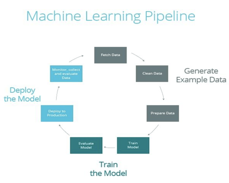
Scope → → Data Engineering → → Modeling → → Deployment → → Monitoring → → Business Analysis → → (Repeat).

Framing the Problem

The way you frame a problem changes its difficulty.

• Case Study: You want to predict which app a user will open next on their phone.
• Approach A (Multiclass Classification): The input is the user state; the output is a probability distribution over all 100 installed apps.
  • Problem: If the user installs a new app, you have to retrain the whole model architecture to add a class.
• Approach B (Regression): The input is (User State + App Feature); the output is a score (0 to 1) of likelihood.
  • Benefit: If a user installs a new app, you just feed its features into the existing model. No retraining required.

Decoupling Objectives

In production, stakeholders have conflicting goals.

• Marketing: Wants to maximize clicks.
• Safety: Wants to minimize spam/NSFW content.
• Engineering: Wants to minimize latency.
  
  
  The Fix: Don't train one model to do everything. Train separate models (one for clicks, one for spam probability) and combine their outputs in the final ranking logic. This allows you to tweak the weighting (e.g., "be stricter on spam today") without retraining the neural networks.

Chapter 3: Data Engineering Fundamentals

This is the chapter data scientists usually skip, and it is the reason their models fail to scale.

Data Formats: The Row vs. Column War

• Row-Major (CSV, JSON, Avro): Data is stored row-by-row.
  • Use Case: fast writes; accessing specific user profiles.
• Column-Major (Parquet, ORC): Data is stored column-by-column.
  • Use Case: Analytical queries (e.g., "What is the average age of all users?").
  • Shocking Efficiency: Converting a CSV to Parquet can often reduce file size by 60-80% and speed up analytical queries by 10x because the system scans contiguous memory.

Data Models

• Relational (SQL): Strict schemas. Great for transactional consistency (banking).
• NoSQL (Document/Graph): Flexible schemas.
  • Graph Databases: Essential for social networks or fraud detection where the relationships (edges) matter more than the data points (nodes).

Processing: The Move to Real-Time

• Batch Processing (MapReduce/Spark): Processing historical data. High throughput, high latency.
• Stream Processing (Kafka/Flink): Processing data as it flows. Low latency.
• The Industry Shift: Companies are moving away from the Lambda Architecture (maintaining two separate pipelines for batch and stream, which causes code duplication and bugs) toward the Kappa Architecture (treating everything as a stream).

Chapter 4: Training Data

"Data is the new code." The code you write (the model architecture) matters less than the data you feed it.

Sampling: It's Not Just random.choice()

• Non-Probability Sampling: Selecting data based on convenience (e.g., the top 100 rows). This introduces massive bias.
• Stratified Sampling: Essential for rare classes. If you are detecting a disease that affects 1% of people, random sampling might give you zero positive cases. Stratified sampling forces the inclusion of rare groups.

Reservoir Sampling: Reservoir Sampling: A critical algorithm for streaming data. How do you select a random sample of k items from a stream of unknown length n ? Reservoir sampling allows you to do this in a single pass with fixed memory.

The Labeling Bottleneck

• Hand Labels: Gold standard, but slow and expensive.
• Natural Labels: Labels inferred from user behavior (e.g., if a user watches a movie for 30 minutes, they "liked" it).
  • Danger: The Feedback Loop Length. In high-frequency trading, you get the label (profit/loss) in milliseconds. In fraud detection, you might not get the label (a chargeback report) for 3 months.
• Weak Supervision (Snorkel): Using heuristics to label data programmatically.
  • Example: Instead of paying doctors to label X-rays, write a function: IF "pneumonia" IN doctor_notes THEN Label = POSITIVE. This is noisy but fast and scalable.

Handling Class Imbalance

When your target class is rare (fraud, click-throughs), accuracy is a lie.

• Resampling:
  • Undersampling: Delete majority class data (fast, but loses information).
  • Oversampling: Duplicate minority class data (risk of overfitting).
  • SMOTE: Synthesize new minority examples by interpolating between existing ones.
• Algorithm-Level: Use Class-Balanced Loss or Focal Loss to tell the model: "Pay 100x more attention to a mistake on the minority class than the majority class."

Chapter 5: Feature Engineering

Feature engineering is how you inject domain knowledge into the model.

Key Techniques

• One-Hot Encoding: Standard for categorical data, but fails if you have 1 million categories (e.g., User IDs).
• Hashing Trick: Hash the category into a fixed vector size. It handles new categories automatically and is memory efficient. Collisions (two categories hashing to the same spot) are surprisingly acceptable in high-dimensional spaces.
• Positional Embeddings: Critical for Transformers. Since neural nets process parallel inputs, you must explicitly tell the model that "Dog bites Man" is different from "Man bites Dog" by embedding the position index.

The Silent Killer: Data Leakage

This causes models to have 99% accuracy in dev and 50% in prod.

1. Scale-After-Split: If you normalize your data (subtract mean, divide by variance) using the entire dataset before splitting, you have leaked information from the test set into the train set.
2. Time-Travel: Using a feature that wouldn't be available at inference time.
   • Example: Using "Duration of Call" to predict "Will Customer Pick Up?". You only know the duration after they pick up.

Chapter 6: Model Development & Offline Evaluation

Don't start with a Transformer. Start with a baseline.

Model Selection

• The SOTA Trap: Just because a model is State-of-the-Art on a leaderboard doesn't mean it's usable. It might be too slow or too large.
• Ensembles:
  
  • Bagging (Random Forest): Trains models independently. Reduces variance. Good for overfitting.
  • Boosting (XGBoost): Trains models sequentially, focusing on previous mistakes. Reduces bias. Good for underfitting.
  • Stacking: Using a "meta-learner" to combine predictions from a Neural Net, a Linear Regressor, and a Tree.

Advanced Evaluation

• Calibration: A model predicting 80% rain should result in rain 80% of the time. Modern Deep Learning models are notoriously overconfident (poorly calibrated). You must use techniques like Platt Scaling to fix this.
• Slice-based Evaluation: Aggregate metrics hide bias. A model with 95% accuracy might have 40% accuracy on a specific minority demographic. You must evaluate performance on specific data slices.
• Perturbation Sensitivity: If changing one pixel in an image changes the classification from "Panda" to "Gibbon" (Adversarial Attack), your model is brittle.
  

Chapter 7: Deployment & Prediction Service

Your model is just a binary file. Serving it is an architectural challenge.

Deployment Patterns

• Model-as-a-Service: Wrap the model in a Docker container (Flask/FastAPI) and expose a REST API.
• Batch Prediction: Run the model once a day, write predictions to a database (Redis/Cassandra).
  • Advantage: High throughput, instant retrieval latency.
  • Disadvantage: Can't react to new user behavior instantly.
• Online Prediction: Run the model on request.
  • Advantage: Personalized to the exact moment.
  • Disadvantage: You have a strict latency budget (e.g., 50ms).

Model Compression (Making it fit)

To run on Edge devices (phones, IoT):

1. Quantization: Convert 32-bit floats (4 bytes) to 8-bit integers (1 byte). Reduces size by 4x, often with negligible accuracy loss.
2. Pruning: Set all "small" weights to zero. This makes the matrix sparse and easier to compress.
3. Knowledge Distillation: Train a tiny "Student" model to mimic a massive "Teacher" model. (e.g., DistilBERT).

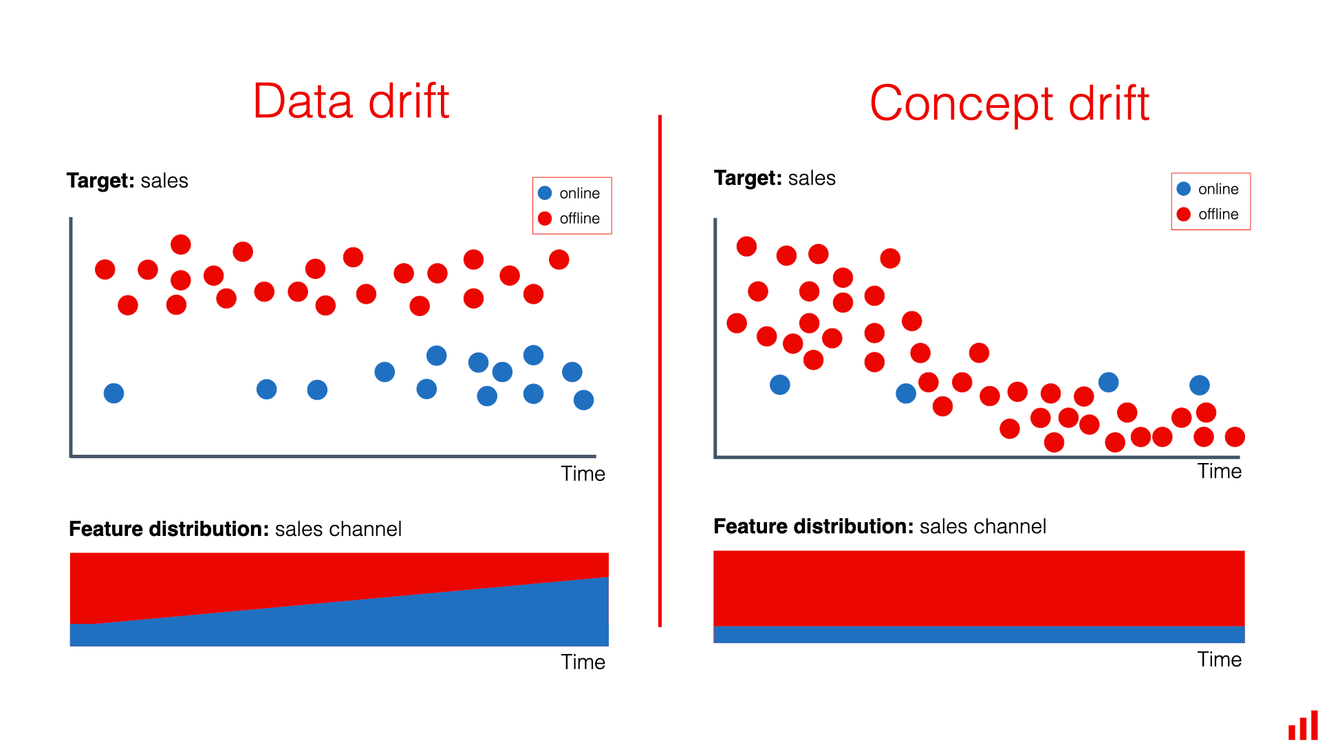
Chapter 8: Data Distribution Shifts & Monitoring

"Software bugs cause crashes. ML bugs cause wrong decisions."

The Three Types of Drift

1. Covariate Shift: The input distribution P ( X ) changes. Example: You trained a face ID model on adults, but now kids are using it. The input features (faces) look different.
2. Label Shift: The output distribution P ( Y ) changes. Example: During a recession, the number of loan defaults skyrockets. The prior probability of "Default" has shifted.
3. Concept Drift: The relationship P(Y∣X) changes. Example: Before 2020, searching "Corona" meant beer. After 2020, it meant virus. The input X is the same, but the mapping to Y changed.

Detecting Drift

• Statistical Tests: Kolmogorov-Smirnov (KS) test or Population Stability Index (PSI).
• Window Size: Choosing the right time window is hard. Too short = false alarms (noise). Too long = slow detection.

Chapter 9: Continual Learning & Testing in Production

Static models are dead models. The Holy Grail is Continual Learning.

Stateless vs. Stateful Retraining

• Stateless: Retrain from scratch every week. Expensive.
• Stateful: Continue training (fine-tuning) the existing model with new data.
  • Risk: Catastrophic Forgetting (The model learns new data but forgets old patterns).
  • Success Story: Grubhub switched to stateful incremental learning, reducing compute costs by 45% and increasing conversion by 20%.

Safe Deployment Strategies

Never just replace V1 with V2.

1. Shadow Deployment: V2 runs in parallel with V1. It processes live requests, but its results are not shown to users. You compare the results silently.
2. Canary Release: Roll out V2 to 1% of users. If metrics look good, expand to 5%, 25%, 100%.
3. A/B Testing: The gold standard for measuring business impact.
4. Bandits (Exploration/Exploitation): An automated A/B test. The system dynamically routes more traffic to the better-performing model. It is more data-efficient than A/B testing.

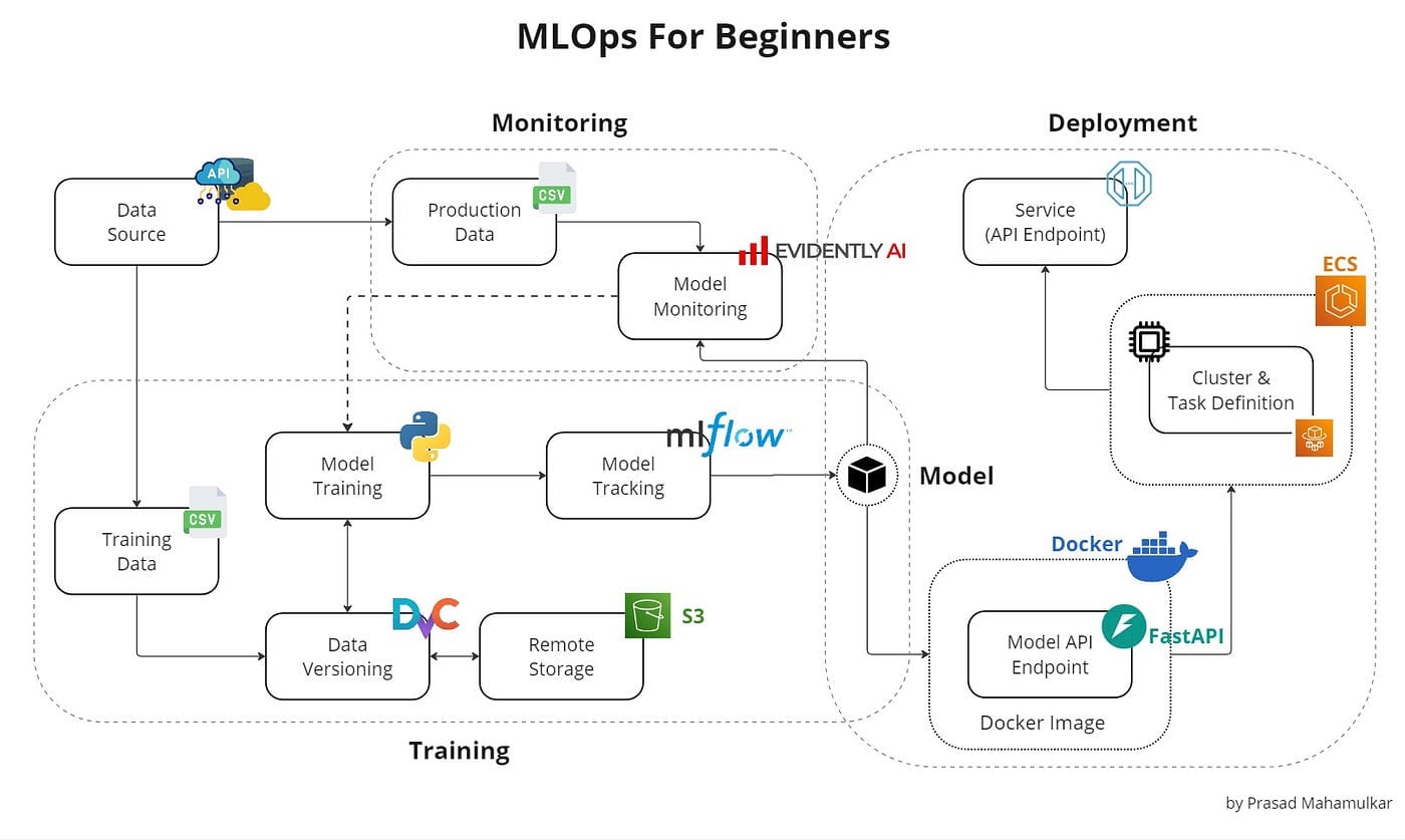
Chapter 10: Infrastructure for MLOps

You can build vs. buy.

• Storage: Data Lakes (S3) for raw data vs. Data Warehouses (Snowflake) for structured data.
• Compute: Elastic clouds (AWS EC2) vs. On-prem.
  • Trend: Cloud Repatriation. Massive companies (like Dropbox) are moving off AWS to private data centers because cloud bills eventually destroy margins.
• Orchestration: Tools like Airflow, Kubeflow, and Metaflow manage the dependency graph of ML tasks.
• The Feature Store: A centralized repository ensuring that the features used for training (batch) are mathematically identical to features used for inference (online). This solves the "training-serving skew."

Chapter 11: The Human Side

Ultimately, ML systems affect people.

UX for ML

• The Uncanny Valley of Latency: Sometimes, a model is too fast. Financial apps sometimes add artificial loading bars because users don't trust a loan approval that happens in 5 milliseconds.
• Consistency: Users prefer a predictable, slightly worse system over a system that behaves erratically.

Responsible AI

• Bias: Bias is not just in the dataset; it is in the choice of objective function.
• Case Study (The UK Grading Fiasco): An algorithm assigned grades to students based on the historical performance of their schools. It famously downgraded high-performing students in poor schools to "maintain the distribution." It optimized for system stability over individual fairness.
• Solution: Model Cards. Similar to nutritional labels on food, every model should have a "Card" listing its intended use, limitations, training data demographics, and bias audit results.

Nutshell:

Designing Machine Learning systems is about trade-offs. It is about trading accuracy for latency, flexibility for maintainability, and complexity for reliability. As Huyen concludes, the best ML engineer isn't the one who knows the most algorithms; it's the one who can build a system that delivers value continuously, safely, and efficiently.

Book Download link