Why XGBoost Dominates? 4 Game-Changing Parameters Explained
XGBoost (eXtreme Gradient Boosting) is one of the most powerful machine learning algorithms, dominating Kaggle competitions and real-world applications. But what makes it "extreme" compared to traditional Gradient Boosting Machines (GBM)?
The answer lies in its optimized parameters, computational efficiency, and regularization techniques. These parameters allow XGBoost to achieve high accuracy, speed, and scalability, making it "extreme" in both performance and flexibility.
Why Parameters Matter in XGBoost
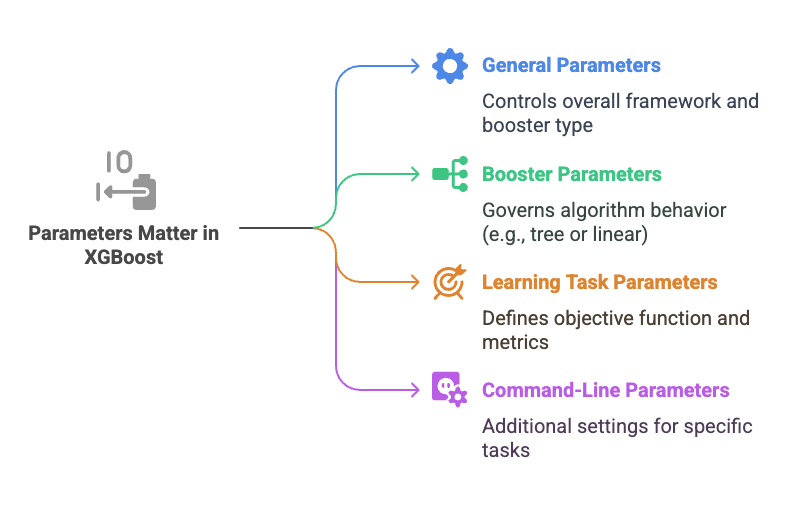
XGBoost’s performance stems from its ability to fine-tune the learning process through a wide range of parameters that control model complexity, learning speed, robustness, and efficiency. These parameters are categorized into:
- General Parameters: Control the overall framework and booster type.
- Booster Parameters: Govern the behavior of the boosting algorithm (e.g., tree or linear booster).
- Learning Task Parameters: Define the objective function and evaluation metrics.
- Command-Line Parameters: Additional settings for specific tasks (e.g., GPU usage).
By carefully tuning these parameters, XGBoost achieves its "extreme" status through:
- Speed: Optimized data structures (DMatrix) and parallel processing.
- Accuracy: Advanced regularization and loss optimization.
- Flexibility: Support for custom objectives and diverse tasks.
- Scalability: Efficient handling of large datasets and distributed computing.
1: General Parameters
These parameters define the high-level configuration of XGBoost.
1. booster
- Description: Specifies the type of booster to use.
- Options:
gbtree: Tree-based booster (default, most common).gblinear: Linear booster for linear models.dart: Dropouts meet Multiple Additive Regression Trees (adds dropout to trees).
- Impact:
gbtreeis typically used for its superior performance on structured data.dartcan improve generalization by introducing randomness, whilegblinearis less common but useful for linear relationships. - Best Practice: Stick with
gbtreeunless you have a specific reason to usedartorgblinear.
2. nthread
- Description: Number of parallel threads for computation.
- Default: Maximum number of threads available.
- Impact: Increases training speed by parallelizing tree construction.
- Best Practice: Leave as default unless you need to limit CPU usage.
3. device
- Description: Specifies the device for computation (e.g., CPU or GPU).
- Options:
cpu(default),cuda(for NVIDIA GPUs). - Impact: Using
cudasignificantly speeds up training on large datasets with compatible hardware. - Best Practice: Use
cudaif you have a compatible GPU; otherwise, stick withcpu.
2: Booster Parameters
These parameters control the behavior of the boosting process, particularly for the gbtree booster, which is the most commonly used.
1. eta (Learning Rate)
- Description: Scales the contribution of each tree.
- Range: [0, 1], typically 0.01–0.3.
- Impact: Lower values make the model more robust by reducing overfitting but require more boosting rounds (
num_boost_round). Higher values speed up training but may lead to overfitting. - Best Practice: Start with 0.1 and tune with cross-validation. Use smaller values (e.g., 0.01) for high accuracy at the cost of longer training.
2. max_depth
- Description: Maximum depth of each tree.
- Range: 1–∞, typically 3–10.
- Impact: Deeper trees capture more complex patterns but increase the risk of overfitting. Shallower trees are simpler and generalize better.
- Best Practice: Start with 6 and adjust based on dataset complexity. Use cross-validation to find the optimal depth.
3. min_child_weight
- Description: Minimum sum of instance weight (Hessian) needed in a child node.
- Range: [0, ∞], typically 1–10.
- Impact: Higher values prevent overfitting by requiring more data to create a split, leading to simpler trees.
- Best Practice: Increase for noisy datasets or when overfitting is observed. Start with 1.
4. subsample
- Description: Fraction of training data sampled for each tree.
- Range: (0, 1], typically 0.5–1.0.
- Impact: Introduces randomness, reducing overfitting and improving generalization. Lower values make the model more robust but may increase training time.
- Best Practice: Use 0.8–1.0 for small datasets, 0.5–0.8 for larger ones.
5. colsample_bytree, colsample_bylevel, colsample_bynode
- Description:
colsample_bytree: Fraction of features used per tree.colsample_bylevel: Fraction of features used per level in a tree.colsample_bynode: Fraction of features used per split.
- Range: (0, 1], typically 0.5–1.0.
- Impact: Adds randomness, reducing overfitting and improving generalization. Lower values increase diversity among trees.
- Best Practice: Start with 0.8 for
colsample_bytreeand adjust others if needed.
6. lambda (L2 Regularization)
- Description: L2 regularization term on weights.
- Default: 1.
- Impact: Reduces overfitting by penalizing large weights, leading to simpler models.
- Best Practice: Increase (e.g., 10) for datasets prone to overfitting. Tune with cross-validation.
7. alpha (L1 Regularization)
- Description: L1 regularization term on weights.
- Default: 0.
- Impact: Encourages sparsity in feature weights, useful for feature selection.
- Best Practice: Use non-zero values (e.g., 0.1–1.0) when feature selection is desired.
8. gamma (Minimum Loss Reduction)
- Description: Minimum loss reduction required to make a split.
- Default: 0.
- Impact: Higher values result in fewer splits, producing simpler trees and reducing overfitting.
- Best Practice: Start with 0 and increase (e.g., 0.1–1.0) for complex datasets.
9. num_boost_round
- Description: Number of boosting iterations (trees).
- Default: 10 (but typically set higher, e.g., 100–1000).
- Impact: More rounds increase model complexity and training time. Combine with early stopping to avoid overfitting.
- Best Practice: Use a high value (e.g., 1000) with early stopping to let the model determine the optimal number.
3: Learning Task Parameters
These parameters define the objective function and evaluation metrics.
1. objective
- Description: Specifies the learning task and loss function.
- Common Options:
reg:squarederror: Squared loss for regression.binary:logistic: Logistic loss for binary classification.multi:softmax: Softmax for multiclass classification.rank:pairwise: Pairwise ranking for ranking tasks.
- Impact: Determines the type of problem XGBoost solves.
- Best Practice: Choose based on the task (e.g.,
binary:logisticfor binary classification).
2. eval_metric
- Description: Metric for evaluating model performance.
- Common Options:
rmse: Root mean squared error (regression).mae: Mean absolute error (regression).logloss: Log loss (classification).mlogloss: Multiclass log loss.auc: Area under the ROC curve.
- Impact: Guides model optimization and early stopping.
- Best Practice: Match the metric to the task (e.g.,
aucfor imbalanced classification).
3. scale_pos_weight
- Description: Balances positive and negative classes in imbalanced datasets.
- Default: 1.
- Impact: Adjusts the weight of positive class to handle imbalance (e.g.,
sum(negative)/sum(positive)). - Best Practice: Set based on class imbalance ratio for binary classification.
4: What Makes XGBoost "Extreme"?
The "extreme" in XGBoost comes from its ability to leverage these parameters for:
- Speed:
- Parallel tree construction (
nthread). - GPU acceleration (
device=cuda). - Optimized data structure (DMatrix).
- Parallel tree construction (
- Accuracy:
- Regularization (
lambda,alpha,gamma) prevents overfitting. - Flexible loss functions (
objective) suit diverse tasks. - Early stopping and cross-validation optimize performance.
- Regularization (
- Scalability:
- Handles large datasets via subsampling (
subsample,colsample_*). - Missing value handling reduces preprocessing needs.
- Handles large datasets via subsampling (
- Robustness:
- Parameters like
min_child_weightandmax_depthbalance bias and variance. scale_pos_weightaddresses imbalanced data.
- Parameters like
XGBoost Parameters Table:
The table below organizes XGBoost parameters into three categories: General Parameters, Booster Parameters (specific to the gbtree booster, the most common), and Learning Task Parameters. Each entry includes the parameter name, description, value range, default value, recommended starting value, and impact on the model.
| Category | Parameter | Description | Value Range | Default Value | Recommended Starting Value | Impact |
|---|---|---|---|---|---|---|
| General Parameters | booster |
Type of booster to use. | gbtree, gblinear, dart |
gbtree |
gbtree |
Determines model type; gbtree excels for structured data, dart adds dropout for generalization, gblinear suits linear relationships. |
nthread |
Number of parallel threads for computation. | Integer ≥ 1 | Max available threads | Max available threads | Speeds up training by parallelizing tree construction. | |
device |
Device for computation (CPU or GPU). | cpu, cuda |
cpu |
cpu (use cuda if GPU available) |
GPU (cuda) accelerates training on large datasets. |
|
| Booster Parameters | eta (learning rate) |
Scales the contribution of each tree. | [0, 1] | 0.3 | 0.1 | Lower values reduce overfitting but require more boosting rounds. |
max_depth |
Maximum depth of each tree. | Integer ≥ 1 | 6 | 4–6 | Deeper trees capture complex patterns but risk overfitting. | |
min_child_weight |
Minimum sum of instance weight (Hessian) needed in a child node. | [0, ∞] | 1 | 1 | Higher values prevent overfitting by requiring more data for splits. | |
subsample |
Fraction of training data sampled per tree. | (0, 1] | 1.0 | 0.8 | Adds randomness, reducing overfitting; lower values improve generalization. | |
colsample_bytree |
Fraction of features used per tree. | (0, 1] | 1.0 | 0.8 | Adds randomness, reducing overfitting and improving diversity. | |
colsample_bylevel |
Fraction of features used per tree level. | (0, 1] | 1.0 | 1.0 | Adds randomness at the level level; use cautiously for complex datasets. | |
colsample_bynode |
Fraction of features used per split. | (0, 1] | 1.0 | 1.0 | Adds randomness at the split level; useful for high-dimensional data. | |
lambda |
L2 regularization term on weights. | [0, ∞] | 1 | 1 | Reduces overfitting by penalizing large weights. | |
alpha |
L1 regularization term on weights. | [0, ∞] | 0 | 0.1 | Encourages sparsity, useful for feature selection. | |
gamma |
Minimum loss reduction required to make a split. | [0, ∞] | 0 | 0.1 | Higher values produce simpler trees, reducing overfitting. | |
num_boost_round |
Number of boosting iterations (trees). | Integer ≥ 1 | 10 | 100–1000 (with early stopping) | More rounds increase complexity; use with early stopping to optimize. | |
| Learning Task Parameters | objective |
Learning task and loss function. | Varies (e.g., reg:squarederror, binary:logistic, multi:softmax) |
reg:squarederror |
Task-dependent (e.g., multi:softmax for multiclass) |
Defines the problem type (regression, classification, ranking). |
eval_metric |
Metric for evaluating model performance. | Varies (e.g., rmse, mae, logloss, mlogloss, auc) |
Depends on objective |
Task-dependent (e.g., mlogloss for multiclass) |
Guides optimization and early stopping; align with task. | |
scale_pos_weight |
Balances positive/negative classes in imbalanced datasets. | [0, ∞] | 1 | sum(negative)/sum(positive) |
Improves performance on imbalanced datasets. |
Practical Example: Applying Parameters
Below is a Python example using the Iris dataset to demonstrate how to set these parameters in XGBoost, using recommended starting values from the table.
import xgboost as xgb
from sklearn.datasets import load_iris
from sklearn.model_selection import train_test_split
from sklearn.metrics import accuracy_score

# Load dataset
iris = load_iris()
X, y = iris.data, iris.target

# Split data
X_train, X_test, y_train, y_test = train_test_split(X, y, test_size=0.2, random_state=42)

# Convert to DMatrix
dtrain = xgb.DMatrix(X_train, label=y_train)
dtest = xgb.DMatrix(X_test, label=y_test)

# Define parameters
params = {
    # General Parameters
    'booster': 'gbtree',
    'device': 'cpu',
    'nthread': -1,  # Use all available threads
    # Booster Parameters
    'eta': 0.1,
    'max_depth': 4,
    'min_child_weight': 1,
    'subsample': 0.8,
    'colsample_bytree': 0.8,
    'colsample_bylevel': 1.0,
    'colsample_bynode': 1.0,
    'lambda': 1.0,
    'alpha': 0.1,
    'gamma': 0.1,
    # Learning Task Parameters
    'objective': 'multi:softmax',
    'num_class': 3,
    'eval_metric': 'mlogloss'
}

# Train model with early stopping
evals = [(dtrain, 'train'), (dtest, 'eval')]
bst = xgb.train(params, dtrain, num_boost_round=100, evals=evals, early_stopping_rounds=10, verbose_eval=False)

# Predict
y_pred = bst.predict(dtest)

# Evaluate
accuracy = accuracy_score(y_test, y_pred)
print(f"Accuracy: {accuracy:.2f}")
Explanation:
- Parameters: The example uses recommended starting values from the table, balancing model complexity and generalization.
- Early Stopping: Stops training if
mloglossdoesn’t improve for 10 rounds, preventing overfitting. - Evaluation: Tracks performance on both training and test sets to ensure robust results.
Best Practices for Parameter Tuning
- Start with Recommended Values: Use the starting values from the table as a baseline.
- Focus on Key Parameters: Prioritize
eta,max_depth,subsample, andcolsample_bytreefor initial tuning. - Use Cross-Validation: Employ
xgb.cvor scikit-learn’sGridSearchCVto validate parameter choices. - Leverage Early Stopping: Set a high
num_boost_round(e.g., 1000) and use early stopping to optimize the number of trees. - Address Imbalance: Calculate
scale_pos_weightfor imbalanced datasets to improve performance. - Tune Incrementally: Adjust one parameter at a time to isolate its impact.
- Monitor Overfitting: Use regularization parameters (
lambda,alpha,gamma) to control model complexity.
Tuning Parameters
Tuning XGBoost parameters is critical for optimal performance. Common approaches include:
- Grid Search: Test all combinations of a parameter grid (slow but thorough).
- Random Search: Sample random combinations (faster, often effective).
- Bayesian Optimization: Use tools like Optuna or Hyperopt for efficient tuning.
Example of grid search using scikit-learn:
from sklearn.model_selection import GridSearchCV
from xgboost import XGBClassifier

# Define model
model = XGBClassifier(objective='multi:softmax', num_class=3)

# Define parameter grid
param_grid = {
    'max_depth': [3, 4, 5],
    'learning_rate': [0.01, 0.1, 0.3],
    'subsample': [0.7, 0.8, 0.9],
    'colsample_bytree': [0.7, 0.8, 0.9]
}

# Perform grid search
grid_search = GridSearchCV(model, param_grid, cv=5, scoring='accuracy')
grid_search.fit(X_train, y_train)

# Best parameters and score
print(f"Best parameters: {grid_search.best_params_}")
print(f"Best accuracy: {grid_search.best_score_:.2f}")
Common Pitfalls
- Overfitting: Avoid overly deep trees (
max_depth) or too many rounds without early stopping. - Underfitting: Ensure
etaisn’t too low andnum_boost_roundis sufficient. - Ignoring Imbalance: Use
scale_pos_weightfor imbalanced datasets. - Over-Tuning: Excessive tuning on small datasets can lead to overfitting to the validation set.
Conclusion
XGBoost’s "extreme" performance is driven by its highly configurable parameters, which balance speed, accuracy, and robustness. By understanding and tuning parameters like eta, max_depth, subsample, and regularization terms, you can tailor XGBoost to a wide range of tasks. The example code provided demonstrates how to apply these parameters in practice. Experiment with these settings, use cross-validation, and leverage tools like grid search to unlock XGBoost’s full potential.
Resources: