TensorFlow Playground: A Visual Guide to Neural Networks for Everyone

Think about how you learned to recognize a cat. Your parents didn't give you a mathematical formula. Instead, they showed you many cats—big ones, small ones, fluffy ones, striped ones. Gradually, your brain identified patterns: pointy ears, whiskers, a certain way of moving. Without realizing it, you built a mental model of "cat-ness."

Neural networks learn exactly the same way. They look at examples, make mistakes, adjust their understanding, and gradually get better. But here's the problem: neural networks are typically invisible. They're buried in code, running on servers, hidden behind complex mathematics. How do you understand something you can't see?

Enter the neural network playground—an interactive, visual tool that lets you watch artificial intelligence learn in real-time. Popular examples include TensorFlow Playground and various Neural Network Playground implementations. These tools transform abstract algorithms into colorful, animated visualizations where you can see exactly what's happening as a machine learns.

This article will demystify neural network playgrounds and explain every concept you'll encounter—from learning rates to regularization, from batch sizes to epochs. Whether you're a curious beginner or a technical professional wanting to understand the fundamentals better, you'll find explanations tailored to your level. By the end, you'll not only understand how these playgrounds work but also grasp the core principles that power modern artificial intelligence.

Link: Click here to open Tensorflow Playground

What is a Neural Network Playground?

A neural network playground is an interactive web-based tool that visualizes how neural networks work. Imagine a flight simulator, but instead of learning to fly a plane, you're learning how AI learns. You don't need to write a single line of code—everything happens through clicking, dragging, and watching the magic unfold on your screen.

The Visual Interface

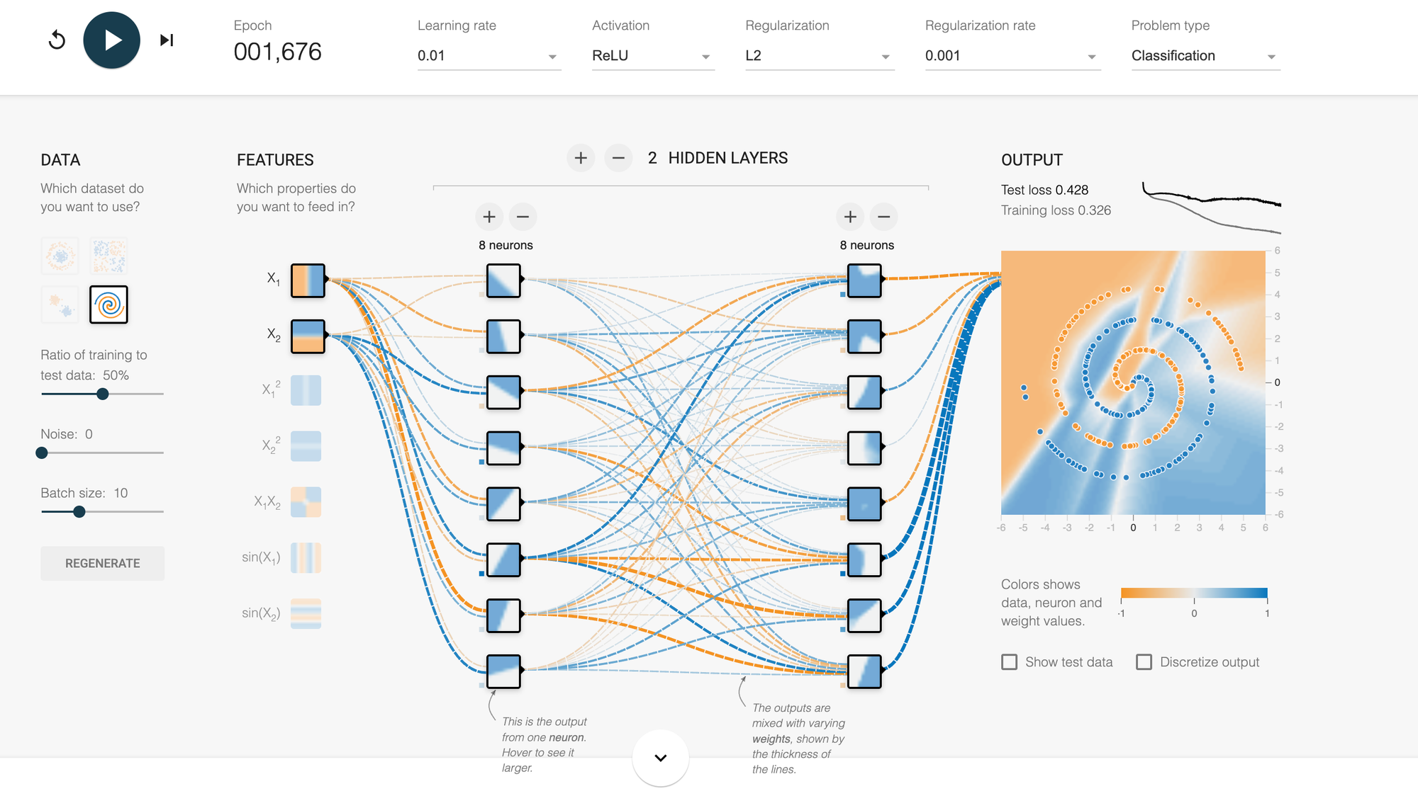
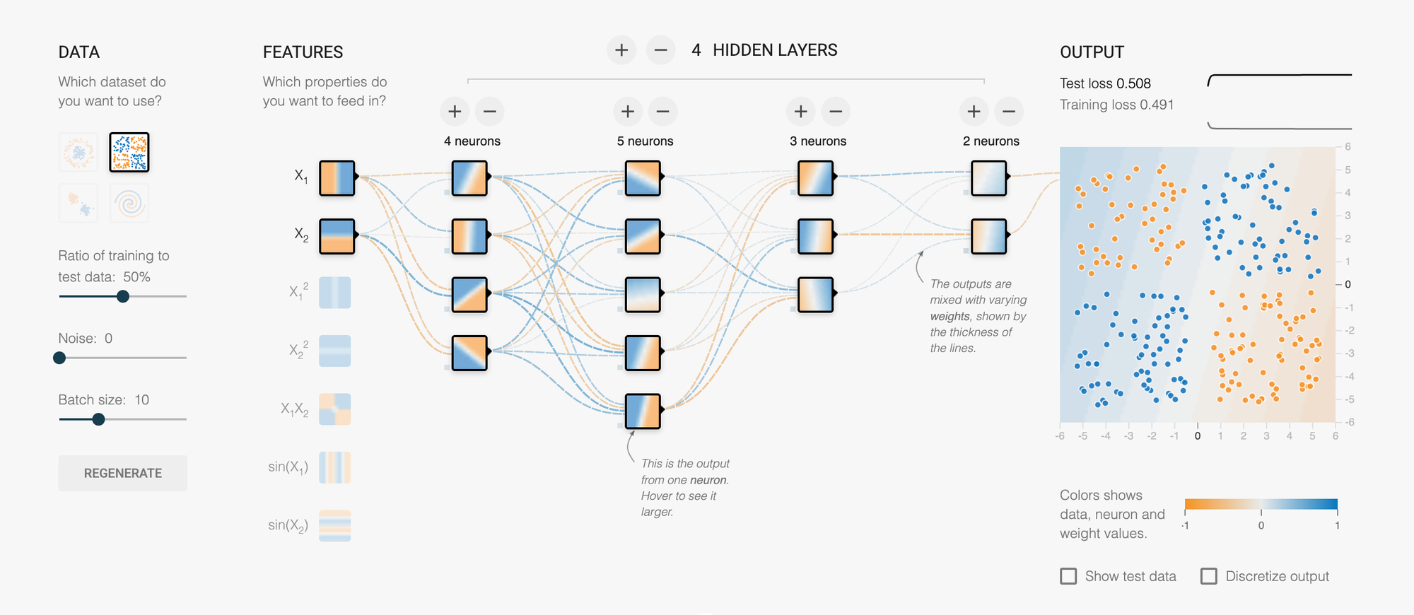
When you open a neural network playground, you typically see several components:

Input Layer: On the left side, you'll see circles representing "features" or characteristics of your data. These might be X₁ and X₂ coordinates—basically, the information your AI starts with.

Hidden Layers: In the middle, you'll see one or more layers of circles (neurons). This is where the actual "thinking" happens. Each circle is like a tiny decision-maker, and together they work to solve the problem.

Output Layer: On the right, you see the final decision or prediction. In classification problems, this determines which category something belongs to.

The Background Canvas: This is perhaps the most mesmerizing part. The entire background shows a color gradient that represents the AI's current understanding. As the network learns, you watch this gradient shift and morph, gradually forming boundaries that separate different types of data.

Link: Click here to open Tensorflow Playground

What Problem Does It Solve?

Most neural network playgrounds tackle classification problems. Picture a field with blue dots and orange dots scattered around. Your job is to draw a boundary that separates blue from orange. Simple, right? But what if the orange dots form a circle surrounded by blue dots? Or a spiral pattern? Suddenly, a straight line won't work.

This is exactly what neural networks do—they learn to draw these boundaries, no matter how complex the pattern. The playground lets you watch this process happen step by step.

Why It's Valuable for Learning

Traditional programming tutorials bombard you with syntax, libraries, and dependencies before you understand what you're building. Neural network playgrounds flip this approach. They give you immediate visual feedback: change a setting, click play, and instantly see how it affects learning. You can break things, experiment wildly, and develop intuition before touching a single line of code.

Think of it as a musical instrument versus sheet music. You could study music theory for years, or you could sit at a piano and start pressing keys. The playground is your piano—a hands-on tool where experimentation leads to understanding.

Core Components Explained

Dataset & Data Points: The Examples We Learn From

Simple Explanation: Data points are the examples your AI studies. Imagine teaching a child to distinguish apples from oranges. You'd show them real fruits—that's your dataset. Each fruit is a data point.

Technical Detail: In the playground, each data point is a feature vector—a set of numerical values that describes something. For a 2D visualization, each point has an X₁ coordinate and an X₂ coordinate. The color (typically blue or orange) represents the label or category we're trying to predict.

The playground offers different dataset patterns:

• Linear/Separable: Two groups separated by a straight line—the easiest problem
• Circle: One group forms a circle inside another—requires non-linear thinking
• XOR (Exclusive OR): Four clusters in a checkerboard pattern—the classic challenge for neural networks
• Spiral: Two spirals intertwined—highly complex, requires sophisticated solutions
• Gaussian Clusters: Random blob-like groupings—mimics real-world messy data

Why do these patterns have different difficulty levels? A straight line can solve linear problems. But try drawing a single straight line to separate a spiral pattern—impossible! Complex patterns require the network to develop more sophisticated understanding, which means more neurons, more layers, and more training time.

Features: The Clues Your AI Uses

Simple Explanation: Features are the characteristics or clues your AI examines to make decisions. When a doctor diagnoses illness, they look at features: temperature, blood pressure, symptoms. When your AI classifies data points, it looks at features like X₁ and X₂ positions.

Technical Detail: Features are input variables fed into the first layer of the network. In the playground, you'll see basic features (X₁, X₂) and engineered features like:

• X₁² and X₂²: Squared values that help recognize curved patterns
• X₁ × X₂: The product of coordinates, useful for diagonal relationships
• sin(X₁) and sin(X₂): Trigonometric functions for wave-like patterns

This is called feature engineering. Sometimes raw data isn't enough. Just as a detective doesn't just record what they see but also notes connections and patterns, neural networks benefit from transformed features that highlight hidden relationships.

Here's the fascinating part: with enough neurons and layers, networks can learn these transformations themselves. But providing pre-engineered features can dramatically speed up learning for complex problems. It's like giving students a formula sheet versus making them derive every formula from scratch.

Hidden Layers & Neurons: The Brain's Architecture

Analogy: Imagine a company making a decision. The CEO doesn't examine every detail personally. Instead, information flows through layers: junior analysts gather data, middle managers synthesize findings, senior executives make strategic calls, and finally, the CEO decides. Each layer adds sophistication and abstraction.
,

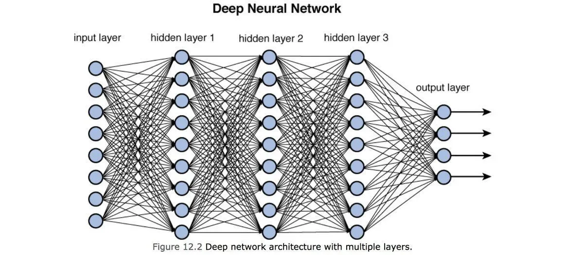
Neural networks work the same way. Each hidden layer processes information from the previous layer, identifying increasingly abstract patterns.

Technical Explanation: Each neuron in a hidden layer receives weighted inputs from the previous layer, sums them up, applies an activation function, and passes the result forward. This is called forward propagation.

The connections between neurons have weights—numbers that get adjusted during learning. A large positive weight means "this input is very important and reinforces my decision." A large negative weight means "this input works against my decision." Near-zero weights mean "this input is irrelevant."

How Many Layers and Neurons?

This is the art of neural network design:

• Too few: The network lacks capacity to learn complex patterns. Like asking an elementary student to solve calculus—they simply don't have the tools.
• Too many: The network memorizes training data instead of learning general patterns (overfitting). Like a student who memorizes every practice problem but can't solve new ones.

Start simple. For linear patterns, one hidden layer with a few neurons suffices. For spirals, you might need 2-3 layers with 4-8 neurons each. The playground lets you experiment and see exactly when adding complexity helps versus when it creates problems.

Learning Rate: The Speed of Learning

Non-Tech Explanation: Imagine you're playing "hot and cold" to find a hidden object. The learning rate determines how big your steps are.

• High learning rate (0.1 - 1): You take giant leaps. Pro: You cover ground fast. Con: You might jump right past the object. Even when you're close, you keep overshooting back and forth.
• Low learning rate (0.0001 - 0.001): You take tiny shuffles. Pro: You're very precise and won't miss the object. Con: It takes forever to get anywhere.
• Just right (0.001 - 0.01): You take medium steps, adjusting to smaller steps as you get warmer.

Technical Detail: Learning rate controls the step size in gradient descent

. During training, the algorithm calculates how wrong the current predictions are (the loss) and which direction to adjust weights. The learning rate determines how much to adjust.

Mathematically: new_weight = old_weight - learning_rate × gradient

Typical ranges:

• 0.00001 - 0.0001: Very conservative, for sensitive or pre-trained models
• 0.001 - 0.01: Common sweet spot for many problems
• 0.1 - 1: Aggressive, risks instability but can work for simple problems

Watch the loss graph in the playground. If it decreases smoothly, your learning rate is good. If it bounces wildly or increases, it's too high. If it barely moves, it's too low. Modern techniques use adaptive learning rates that start high and decrease over time—getting you to the neighborhood quickly, then fine-tuning precisely.

Activation Functions: The Decision Formula

Simple Explanation: After each neuron receives and weighs its inputs, it needs to decide what signal to send forward. The activation function is the rule it uses to make that decision.

Think of it like a light dimmer switch versus an on/off switch. Some activation functions are all-or-nothing (on/off), while others allow gradual responses (dimming).

Technical Explanation: Activation functions introduce non-linearity into neural networks. Without them, stacking multiple layers would be pointless—linear transformations stacked together remain linear.

Common activation functions in playgrounds:

ReLU (Rectified Linear Unit):

• How it works: If input is positive, output equals input. If negative, output is zero.
• Think of it as: A gate that blocks negative signals but passes positive ones unchanged.
• Why popular: Computationally efficient, works well for deep networks, avoids vanishing gradients.

Sigmoid:

• How it works: Squashes any input into a range between 0 and 1.
• Think of it as: A smooth probability converter.
• When to use: Output layer for binary classification (yes/no decisions).
• Downside: Can cause vanishing gradients in deep networks.

Tanh (Hyperbolic Tangent):

• How it works: Similar to sigmoid but outputs between -1 and 1.
• Think of it as: A centered sigmoid, better for hidden layers.
• Advantage: Zero-centered outputs often train faster.

Linear:

• How it works: Output equals input (no transformation).
• When to use: Rarely useful in hidden layers. Sometimes used for regression outputs.
• Limitation: Without non-linear activations, the network can only learn linear relationships.

Here's why this matters: Try solving an XOR problem with only linear activations. It's mathematically impossible! The XOR pattern requires drawing two diagonal boundaries—something linear functions cannot do. Non-linear activations give networks the power to bend, curve, and twist their decision boundaries into complex shapes. See

Regularization: Preventing Memorization

Non-Tech Explanation: Imagine two students preparing for an exam:

Student A studies the concepts, understands the principles, and can solve variations of practice problems. Student B memorizes every practice problem word-for-word but panics when the test has slightly different questions.

Student B has "overfit" to the practice problems. Regularization prevents your neural network from being Student B.

Technical Detail: Regularization adds a penalty for complexity to the loss function. It tells the network: "Don't just minimize errors—also keep your weights small and simple."

L1 Regularization (Lasso):

• Adds the sum of absolute weight values to the loss
• Tends to drive some weights exactly to zero
• Effect: Creates sparse networks, essentially performing feature selection
• Like Marie Kondo for neural networks—removes connections that don't "spark joy"

L2 Regularization (Ridge):

• Adds the sum of squared weight values to the loss
• Prefers many small weights over few large ones
• Effect: Distributes importance across features rather than relying heavily on a few
• The most commonly used regularization

Regularization Rate: A number (typically 0 to 0.1) controlling how much penalty to apply.

• 0: No regularization—network can memorize freely
• 0.001 - 0.01: Gentle encouragement to stay simple
• 0.1+: Strong simplification pressure—might underfit

In the playground, watch what happens to complex problems:

• No regularization: The decision boundary might wiggle through every single training point, creating a convoluted mess.
• With regularization: The boundary stays smooth and general, even if it misclassifies a few training points. This actually improves performance on new data!

Batch Size: How Many Examples at Once?

Simple Explanation: Imagine learning vocabulary:

• Method 1: Study one word, test yourself, adjust your strategy, repeat. Very responsive but time-consuming.
• Method 2: Study all 100 words, then test yourself once. Efficient but you won't adjust your approach until the end.
• Method 3: Study 10 words at a time, test, adjust, repeat. Balanced approach.

Batch size determines how many examples the network looks at before updating its weights.

Technical Detail: During training, the network processes data in batches. After each batch, it calculates the average error and adjusts weights.

Batch Size = 1 (Online Learning):

• Updates after every single example
• Pro: Adapts quickly, can escape local minima more easily
• Con: Noisy, computationally inefficient, updates are less stable
• Training graph: Jagged, jumpy loss curve

Batch Size = 10-32 (Mini-Batch):

• The modern standard and default for most applications
• Pro: Balance between speed and stability, better gradient estimates
• Con: Requires tuning to find the right size
• Training graph: Smooth descent with minor fluctuations

Batch Size = All Data (Batch Gradient Descent):

• Updates once per epoch after seeing all examples
• Pro: Stable, smooth updates, precise gradient direction
• Con: Slow, memory-intensive, can get stuck in local minima
• Training graph: Very smooth but slow improvement

In playgrounds with small datasets, batch size might seem irrelevant. But understanding it prepares you for real-world scenarios where you're training on millions of examples. There, batch size becomes crucial for balancing memory constraints, training speed, and convergence quality.

Epochs: How Many Times to Study

Non-Tech Explanation: An epoch is one complete pass through all your training data. If you have 100 examples and the network sees all 100 once, that's one epoch.

Why multiple epochs? Think about studying a textbook. You don't read each page once and call yourself an expert. You review multiple times, each pass deepening your understanding.

Technical Detail: During each epoch, the network sees every training example (in batches), calculates errors, and adjusts weights. More epochs generally mean more learning, but with diminishing returns and risks.

Early epochs: The network makes rapid progress. It's learning obvious patterns. The loss drops quickly.

Middle epochs: Learning slows. The network is fine-tuning, discovering subtle patterns.

Late epochs: Danger zone. On training data, performance might still improve. But on test data, performance can degrade—the network is starting to memorize rather than generalize.

When to stop?

• Too few epochs: Underfitting—the network hasn't learned enough
• Too many epochs: Overfitting—the network has memorized training quirks
• Just right: When test error stops improving (early stopping)

In playgrounds, you'll often see training run for 100-1000 epochs. Watch the loss curve and the test data performance. The sweet spot is usually when test performance plateaus, even if training performance could still improve.

Noise: The Real-World Messiness

Simple Explanation: In a perfect world, all your data would be clean and precise. In reality, sensors malfunction, people mistype, and measurements have errors. Noise represents this real-world imperfection.

In the playground, adding noise means randomly shifting data points from their "true" positions. It's like asking the network to recognize patterns through a foggy window.

Technical Detail: Noise is typically Gaussian (normally distributed) random values added to features. A noise level of 10 means each coordinate might shift by a random value drawn from a bell curve centered at zero with a standard deviation proportional to the noise level.

Why add noise deliberately?

1. Robustness testing: Can your network still work when data is imperfect?
2. Regularization effect: Noise forces the network to learn broader patterns rather than exact positions.
3. Real-world preparation: Production data will be noisy; training with noise prepares the network.

Watch what happens in the playground when you add noise to a linear pattern. The clean separation becomes fuzzy. The network must learn to look past individual variations and identify the underlying trend. This is exactly what you want—a model that handles messy reality, not just pristine examples.

Training vs. Test Data: The Honest Assessment

The Core Concept: Imagine a teacher who tests students only on problems they've already seen during practice. Great scores? Meaningless. The true test is new, unseen problems.

Neural networks face the same challenge. Training data is what the network learns from. Test data is what we use to honestly assess whether it truly learned or just memorized.

The Split: Typically 70-80% training data, 20-30% test data. The split is random but fixed—test data must never contaminate training.

What to watch in the playground:

• Training loss: Should decrease steadily—this shows the network is learning the training examples.
• Test loss: Should also decrease, ideally tracking close to training loss—this shows the network is generalizing.

The danger signs:

• Training loss keeps decreasing, test loss increases: Classic overfitting. The network is memorizing training data.
• Both losses high: Underfitting. The network hasn't learned enough (needs more capacity, more epochs, or better features).
• Large gap between training and test loss: The network is too focused on training specifics. Add regularization.

This separation between training and testing is fundamental to all machine learning. In the playground, you can visualize both datasets simultaneously—training points are solid, test points are outlined. Watch how the decision boundary tries to satisfy training data while maintaining generalization to test data.

How Everything Works Together: The Training Process

Let's walk through what happens when you click that "play" button and watch the neural network learn:

Step 1: Random Initialization The network starts completely ignorant. All weights are assigned small random values. The initial decision boundary is essentially random—you'll see a chaotic color pattern that makes no sense.

Step 2: Forward Propagation The network takes a batch of training examples. Each data point flows through the layers:

• Input layer receives the features (X₁, X₂, maybe engineered features)
• Each hidden layer neuron calculates a weighted sum of inputs, applies its activation function, and passes the result forward
• The output layer produces a prediction: "I think this point is blue" or "I think it's orange"

Step 3: Calculate Loss The network compares its predictions to the actual labels. Wrong predictions contribute to the loss (error). This number quantifies how badly the network is performing.

Step 4: Backpropagation Here's where the magic happens. The algorithm calculates how much each weight contributed to the error. It's like tracing blame backward: "The output was wrong, so these final layer weights need adjustment. Those weights received their inputs from the previous layer, so those weights also need tweaking." This ripples backward through all layers.

Step 5: Weight Update Using the calculated gradients and the learning rate, weights are adjusted:

• Weights that made predictions worse are decreased
• Weights that made predictions better are increased
• The learning rate controls how aggressive these adjustments are

Step 6: Repeat The network processes the next batch, and the cycle continues. With each iteration, weights inch closer to values that correctly classify the data.

Visualizing the Process:

As this happens hundreds of times per epoch, you watch the background color gradient evolve. Initially chaotic, it gradually forms structure. Boundaries emerge, sharpen, and stabilize. It's like watching evolution in fast-forward—order emerging from randomness through iterative selection pressure.

The loss graph tells the numerical story. A smoothly descending curve means learning is on track. Plateaus [no progress in learning] mean the network has found a good solution or needs more capacity. Wild oscillations mean the learning rate is too high. An increasing curve means something is seriously wrong.

The test data points remain stationary throughout, never influencing training directly. But they're your reality check. If the decision boundary evolves to classify training data perfectly but wildly misclassifies test data, you've overfit. The colors might look beautiful on training points but fail the honesty test.

Practical Experiments to Try

Theory is nothing without practice. Here are five experiments to run in any neural network playground. Each one will teach you something fundamental about how these systems learn.

Experiment 1: Start Simple (The Linear Confidence Builder)

Setup:

• Choose the linear/separable dataset
• One hidden layer with 2-3 neurons
• Learning rate: 0.01
• No regularization
• ReLU activation
• 0 Noise
  

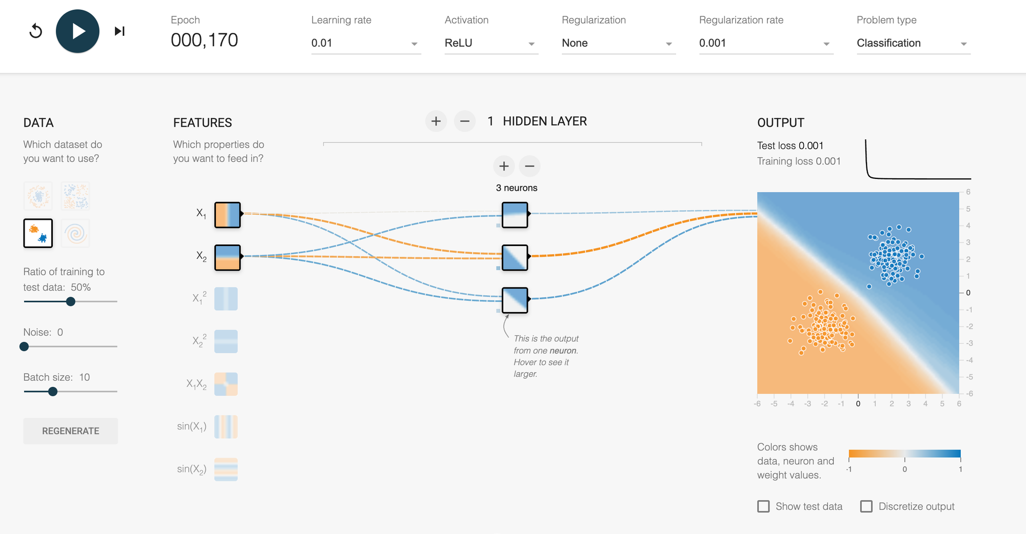
What to watch: The network should solve this quickly—within 20-50 epochs. The decision boundary will be nearly a straight line, cleanly separating the two groups.

Lesson: For simple problems, simple networks suffice. This builds your confidence that these tools actually work.

Try varying: Increase neurons to 8. Does it solve faster? Probably not—it's already an easy problem. You're just adding unnecessary complexity.

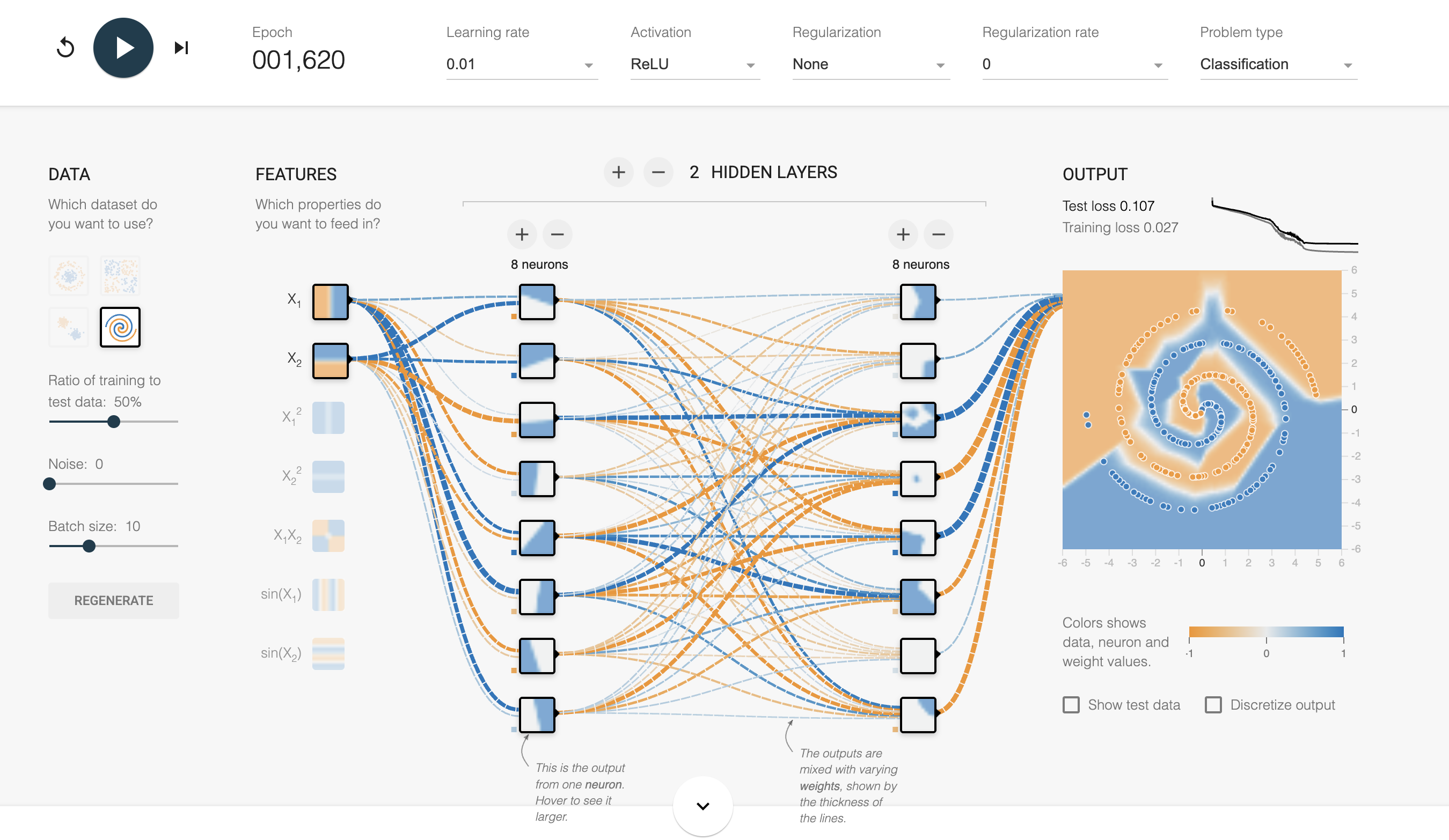
Experiment 2: Face Complexity (The Spiral Challenge)

Setup:

• Choose the spiral dataset
• Start with one hidden layer, 4 neurons
• Learning rate: 0.03
• No regularization
• ReLU activation
• 0 Noise

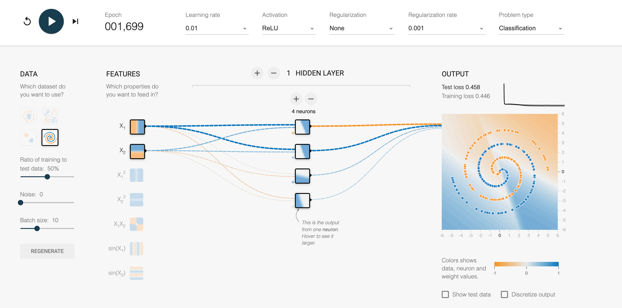
What to watch: The network will struggle. The decision boundary won't form proper spirals.

Now adjust: Add a second hidden layer with 6 neurons. Add a third layer with 4 neurons. Suddenly, the spirals begin to emerge! The network discovers it needs hierarchical feature detection.

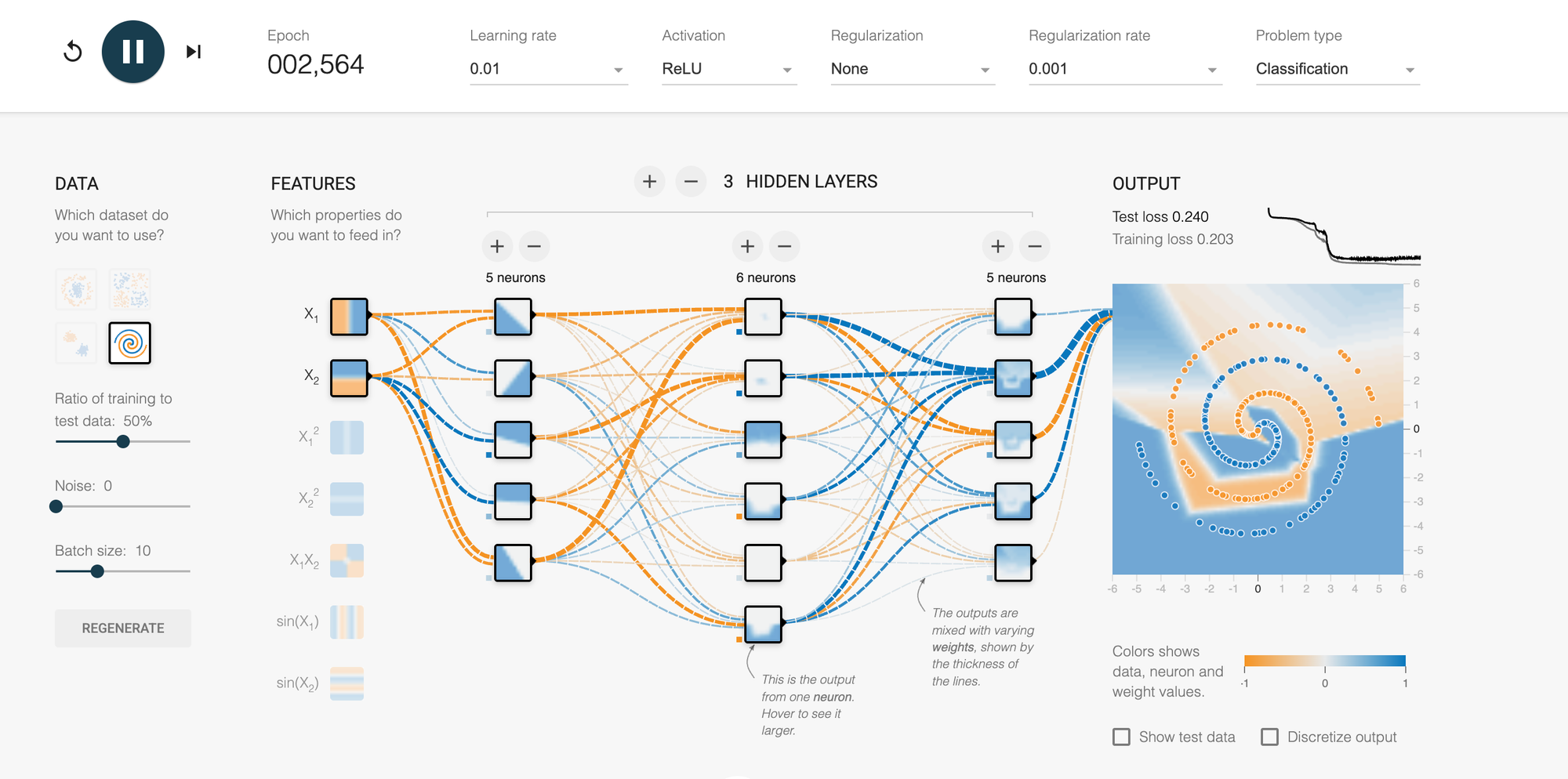
Lesson: Network architecture must match problem complexity. Deep networks aren't just for show—they're necessary for complex patterns.

Experiment 3: The Learning Rate Dance

Setup:

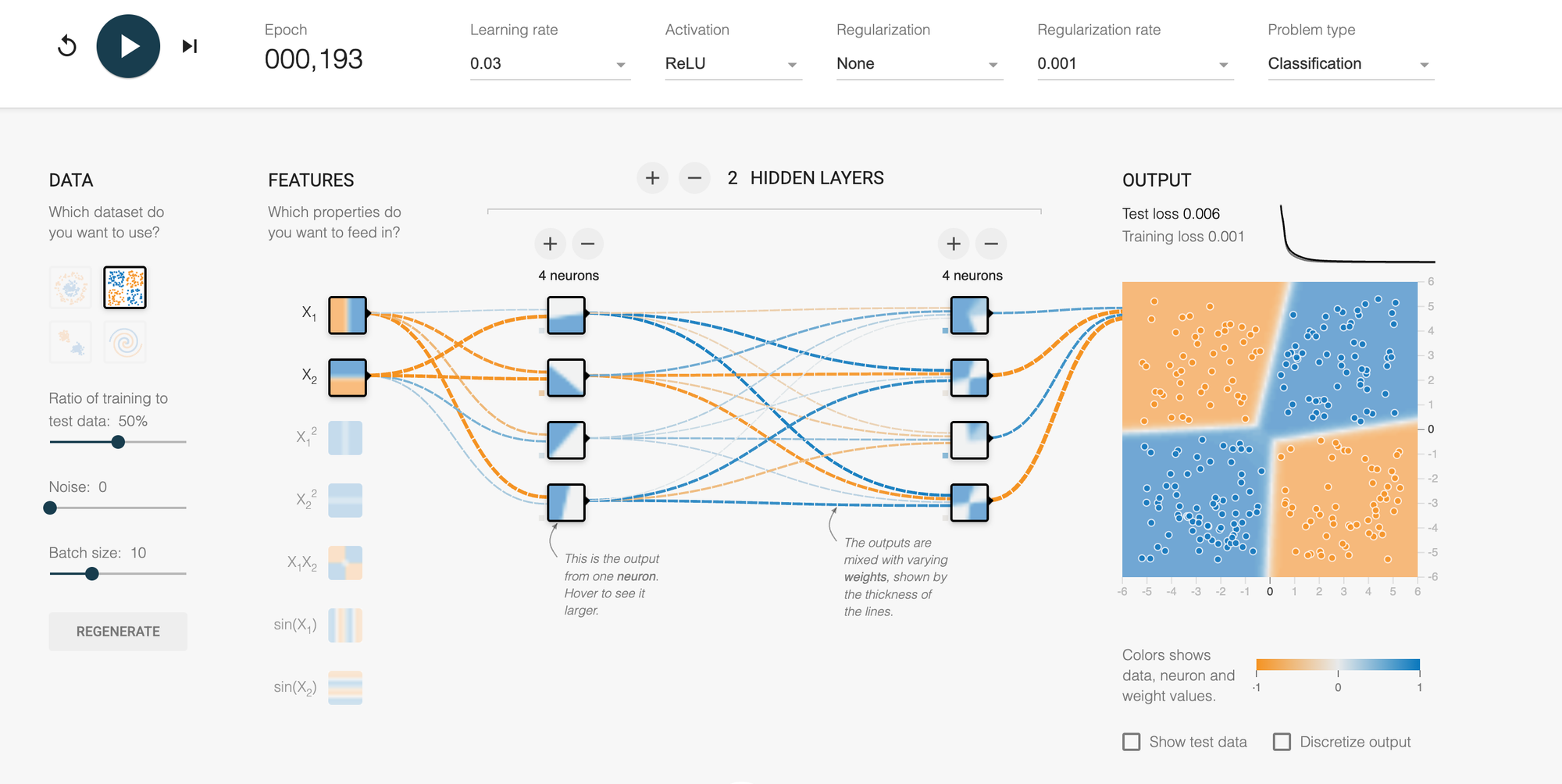
• Choose the XOR dataset
• 2 hidden layers, 4 neurons each
• Try three separate runs with learning rates: 0.001, 0.03, 0.5
• Activation: ReLU

What to watch:

• 0.001: Painfully slow. After 200 epochs, it's still trying to figure things out.
• 0.03: Smooth descent. Decision boundary forms nicely within 100 epochs.
• 0.5: Chaos! The loss bounces around. The boundary oscillates wildly and might never converge.

Lesson: Learning rate is your first tuning knob. Too conservative wastes time. Too aggressive prevents convergence. Finding the sweet spot is essential.

Experiment 4: Regularization's Protective Power

Setup:

• Choose circle dataset (no noise initially)
• 2 hidden layers with 8 neurons each (powerful enough to overfit)
• Learning rate: 0.01
• Run 200+ epochs until you see training loss near zero

First run: No regularization (both L1 and L2 = 0) Second run: L2 regularization = 0.001 Third run: L2 regularization = 0.01

What to watch:

• No regularization: Watch the loss curves carefully. Training loss drops to nearly zero, but test loss may plateau or even increase after initial improvement. The decision boundary fits training data very closely, creating tight curves around training points.
  

• L2 = 0.001: Training loss won't drop quite as low (it's being penalized for complex weights), but test loss stays closer to training loss. The decision boundary is smoother.
• L2 = 0.01: Training loss drops even more slowly and may not reach as low, but the gap between training and test performance shrinks. The boundary becomes noticeably smoother and more generalizable.

Key observation: Compare the final test loss across all three runs. With proper regularization, even though training loss is higher, test loss should be lower—that's better generalization!

Lesson: Regularization trades perfect training performance for better real-world performance. It's your insurance against overfitting, preventing the network from becoming too confident in its training data.

Experiment 5: Batch Size Dynamics

Setup:

• Choose Gaussian dataset
• 2 hidden layers, 4 neurons each
• Learning rate: 0.03
• Run three experiments with batch sizes: 1, 10, all

What to watch:

• Batch size 1: The loss curve is jagged and noisy, but it can escape bad spots quickly. Training takes more iterations.
• Batch size 10: Smooth descent. The sweet spot for most applications.
• Batch size = all: Very smooth curve but slower progress. Each epoch takes longer to compute.

Lesson: Batch size affects the texture of learning. Smaller batches provide noisier but more frequent updates. Larger batches are more stable but less adaptive.

Common Mistakes & How to Fix Them

Even with visualization, you'll encounter frustrating moments. Here's how to diagnose and fix the most common issues:

Problem: The Model Isn't Learning At All

Symptoms: Loss stays high and flat. The decision boundary barely changes even after hundreds of epochs.

Diagnosis:

1. Learning rate too low: Try increasing by 10x
2. Not enough network capacity: Add more neurons or layers
3. Wrong activation function: If you're using linear activations, switch to ReLU or tanh
4. Problem is too hard for current architecture: For spirals, you need at least 2-3 hidden layers

Fix: Start by doubling your learning rate. If that doesn't work, add a hidden layer. The playground makes this easy to test iteratively.

Problem: Training Works But Test Performance Is Terrible

Symptoms: Training loss decreases nicely, but test loss increases or stays high. The decision boundary fits training data perfectly but looks overcomplicated.

Diagnosis: Classic overfitting. Your network has memorized training data rather than learned general patterns.

Fix:

1. Add L2 regularization (start with 0.001)
2. Reduce network complexity (fewer layers or neurons)
3. Stop training earlier (fewer epochs)
4. Add more training data if possible
5. Add noise to training data to make it learn robust features

Problem: Training Is Incredibly Slow

Symptoms: After 500 epochs, you're barely making progress. The loss decreases but at a glacial pace.

Diagnosis: Learning rate is too conservative.

Fix: Increase learning rate. Try multiplying by 3-5. Watch the loss curve—if it starts oscillating, you've gone too far. Back off slightly.

Technical note: In real applications, you'd use adaptive learning rates (Adam, RMSprop) that start high and decrease automatically. Playgrounds typically use simple stochastic gradient descent, so you control this manually.

Problem: Training Is Unstable and Erratic

Symptoms: Loss jumps up and down wildly. The decision boundary flickers chaotically. Sometimes training "explodes" with loss shooting to infinity.

Diagnosis: Learning rate is too high, or you've hit a numerical instability.

Fix:

1. Decrease learning rate by half or more
2. If using sigmoid/tanh, check for vanishing gradients—switch to ReLU
3. Add regularization to stabilize weight updates
4. Reduce batch size for smoother gradient estimates

Problem: The Network Gives Up Too Early

Symptoms: Loss decreases rapidly, then plateaus at a non-optimal solution. The decision boundary is approximately correct but not refined.

Diagnosis: Local minimum or suboptimal initialization.

Fix:

1. Click "regenerate" to restart with different random weights
2. Increase learning rate slightly to help escape the plateau
3. Add momentum (if your playground supports it) to push through flat regions
4. Try a different activation function
5. Adjust network architecture—sometimes one more neuron makes the difference

Real-World Applications: From Playground to Production

The concepts you're experimenting with in the playground power transformative real-world systems. Here's how these abstract dots and gradients translate to technologies you use daily:

Spam Detection: Email providers train neural networks on millions of examples of spam and legitimate emails. Features might include word frequencies, sender information, and header patterns. The network learns a decision boundary separating "spam" from "not spam." Your playground's XOR problem? That's similar to catching spam that uses clever tricks to look legitimate in some ways (legitimate-looking sender but spam content).

Image Recognition: When your phone recognizes faces, it's using deep neural networks—essentially, elaborate versions of your playground with many more layers and neurons. Each layer detects increasingly complex features: edges, then shapes, then facial features, then specific faces. The playground's spiral dataset mirrors this challenge—recognizing patterns that are obvious to humans but require hierarchical feature detection for machines.

Medical Diagnosis: Doctors use AI systems trained on thousands of medical images to detect tumors, disease markers, and anomalies. These networks balance sensitivity (catching actual cases) with specificity (avoiding false alarms)—exactly the precision-recall tradeoff you see when adjusting regularization in the playground.

Recommendation Systems: Netflix, Spotify, and Amazon use neural networks to predict what you'll like. Your features are viewing history, ratings, and demographics. The network learns complex patterns like "people who watch X and Y usually love Z, but only if they're between ages A and B." This is the multi-dimensional version of your playground's classification tasks.

Autonomous Vehicles: Self-driving cars use neural networks to classify objects (is that a pedestrian, another car, or a shadow?), predict trajectories, and make decisions. The networks are massive and trained on millions of miles of data, but the fundamentals—features, layers, activation functions, learning rates—are identical to what you're manipulating in the playground.

The jump from playground to production involves scale (millions of examples vs. hundreds), complexity (hundreds of layers vs. a few), and specialized architectures (convolutional networks, recurrent networks, transformers). But the conceptual foundations remain the same. Master the playground, and you understand the essence of modern AI.

Conclusion: Your Journey from Observer to Practitioner

The playground has shown you that artificial intelligence isn't mystical or incomprehensible. It's pattern recognition through structured learning, visualized through colorful gradients and animated decision boundaries. You understand the vocabulary: features, activations, gradients, regularization. You've seen the dynamics: how learning rate affects convergence, how regularization prevents overfitting, how architecture enables complexity.

Most importantly, you've moved from consumer to creator. You're no longer just using AI—you understand how it works, why it succeeds, and why it fails. In an increasingly AI-driven world, this understanding is power.

Now go forth and experiment. Those colorful dots are waiting to teach you something new 😄