Why XGBoost Outperforms Deep Learning in the Real World
The Secret Weapon of Data Scientists! Learn How This Algorithm Crushes Competitions & Solves Real-World Problems Like a Boss.

XGBoost (eXtreme Gradient Boosting) is one of the most powerful machine learning algorithms today. It consistently wins Kaggle competitions, outperforms traditional models, and is widely used in industry applications—from fraud detection to recommendation systems.
Traditional machine learning models like decision trees and random forests are easy to understand, but they often don’t perform well on complex datasets. XGBoost, short for eXtreme Gradient Boosting, is a powerful and advanced algorithm built for speed, accuracy, and high performance. It’s widely used in real-world applications where getting the best results matters.
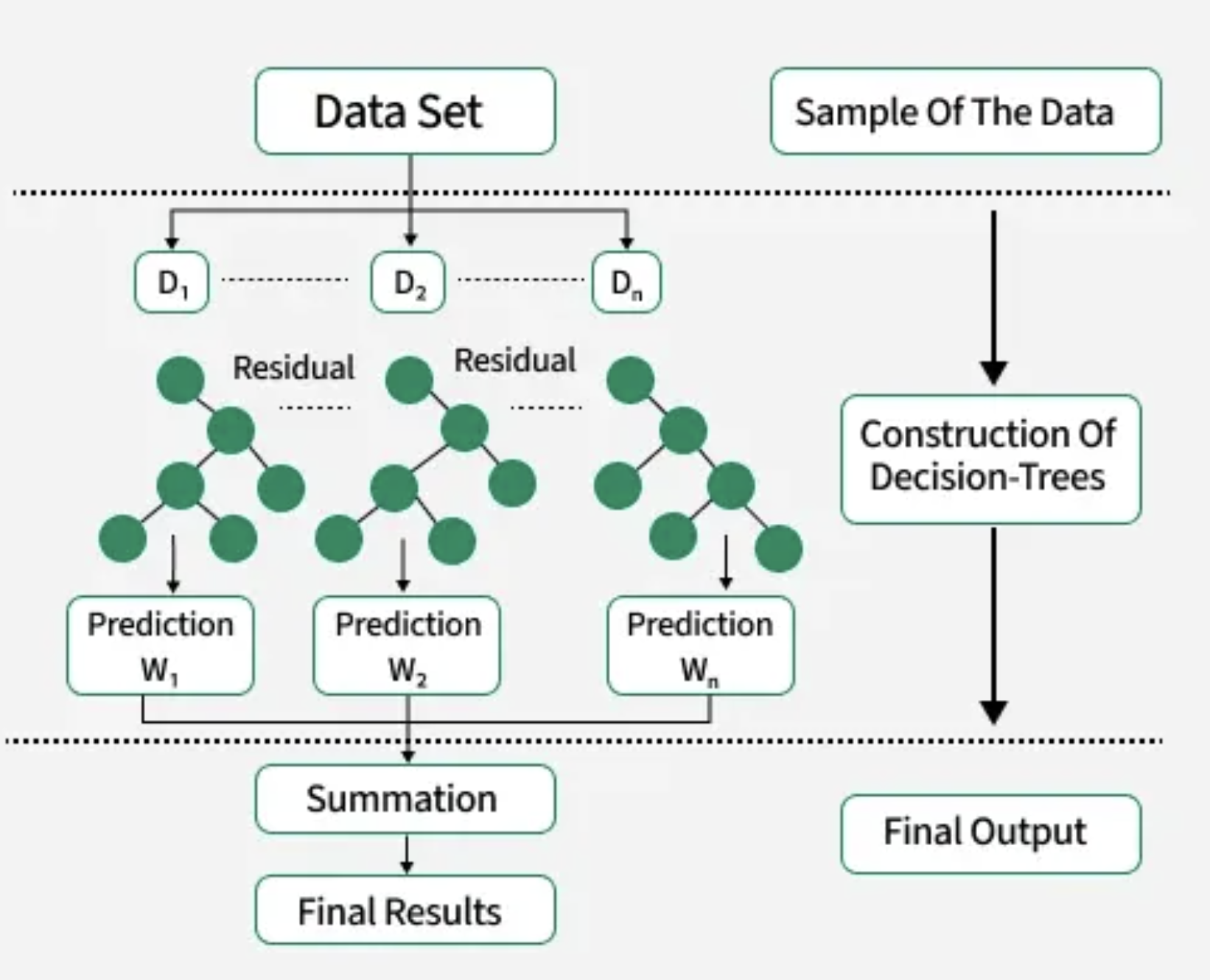
It is an optimized version of the Gradient Boosting algorithm. It’s a type of ensemble learning method, which means it combines many weak models (like small decision trees) to build one strong and accurate model.
In XGBoost, each new decision tree is trained to fix the mistakes made by the previous ones. This step-by-step improvement is called boosting. The algorithm also supports parallel processing, which means it can train on large datasets quickly. Plus, it offers many tuning options, so users can customize the model to suit their specific problem and get the best results.

🧠 How Does XGBoost Work?
XGBoost builds decision trees one after another, where each new tree tries to fix the mistakes made by the previous ones. Here’s a step-by-step breakdown:
- Start with a base model: XGBoost begins with a simple prediction — usually the average of the target values in regression problems. This is the initial guess for every input.
- Calculate the errors (residuals): After this base prediction, the algorithm computes the difference between the actual values and predicted values. These differences are called residuals and show what the model got wrong.
- Train a tree to fix the errors: A new decision tree is trained specifically to predict these residuals — the parts the base model missed.
- Add the correction: The predictions from this tree are added to the previous prediction, improving the overall output.
- Repeat the process: More trees are added one by one, with each tree learning to fix the remaining errors from the last prediction.
- Final prediction = base prediction + sum of all residual corrections:
The final output is not the average of all trees but the initial prediction plus the combined corrections from all the trees.
In XGBoost, residuals refer to the difference between the true values and the predicted values at a given iteration of boosting. They are a key part of how boosting works. Residuals = "What's left to learn" after a prediction.
A simple, step-by-step numeric example of how XGBoost works — using a regression task like predicting house price.
🏠 Problem: Predict House Price
Let’s say the actual house price is: ₹3,600
Step-by-Step XGBoost Prediction:
1️⃣ Initial prediction (Tree 1):
- XGBoost starts with a base prediction, like the average house price from training data.
- Initial Prediction = ₹3,200
- Error (Residual) = ₹3,600 - ₹3,200 = ₹400
2️⃣ Train Tree 2 on residual (₹400):
- Tree 2 tries to predict this error.
- Let’s say Tree 2 learns to predict: ₹250
- Updated Prediction = ₹3,200 + ₹250 = ₹3,450
- New Residual = ₹3,600 - ₹3,450 = ₹150
3️⃣ Train Tree 3 on new residual (₹150):
- Tree 3 learns to correct the remaining error.
- Tree 3 predicts: ₹120
- Updated Prediction = ₹3,450 + ₹120 = ₹3,570
- Residual = ₹3,600 - ₹3,570 = ₹30
4️⃣ Train Tree 4 on new residual (₹30):
- Tree 4 predicts: ₹25
- Final Prediction = ₹3,570 + ₹25 = ₹3,595
✅ Final Output:
- Actual Price = ₹3,600
- XGBoost Predicted = ₹3,595
- Very close!
🧠 Key Point:
- Each tree learns only to fix what the previous tree got wrong, not the entire value.
- So the final prediction = base prediction + sum of small corrections (from all trees).
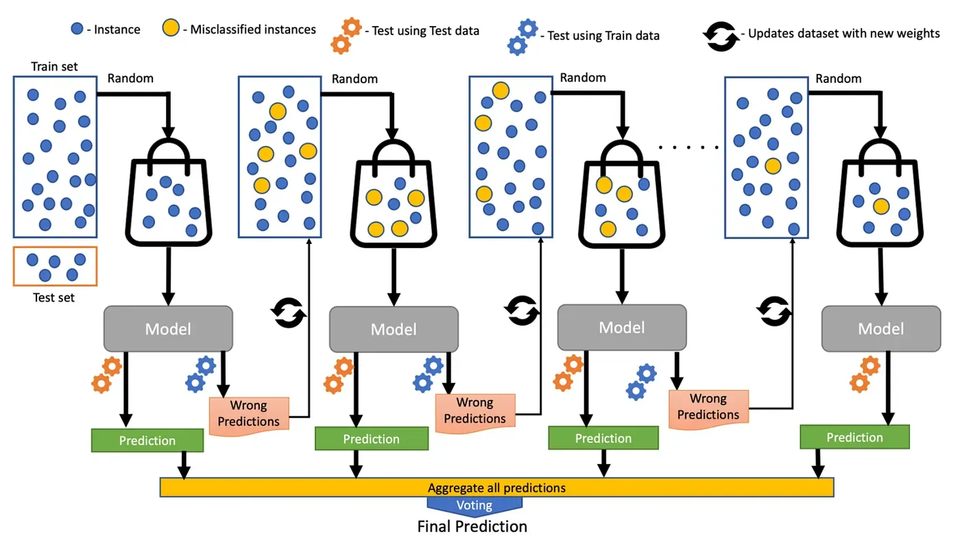
How is it different from Random Forest
| Feature | Random Forest | XGBoost |
|---|---|---|
| Tree Building | All trees built independently | Trees built one after another |
| Learning Method | Bagging | Boosting (Gradient Descent) |
| Goal | Reduce variance | Reduce bias and improve accuracy |
| Speed | Slower for large datasets | Highly optimized for speed |
| Use Case | Easy to use, good baseline | More powerful, but needs tuning |
A Quick Python project:
What We're Doing:
We're building and comparing three different machine learning algorithms to predict loan approval amounts for bank applicants. Using a synthetic dataset of 10,000 loan applications, we train and evaluate:
- XGBoost (Gradient Boosting)
- Random Forest (Ensemble Learning)
- Decision Tree (Single Tree)
Dataset Features:
- Input Variables: Age, Income, Credit Score, Debt-to-Income Ratio, Employment Years, Existing Loans, Delinquencies, Savings Account
- Target Variable: Loan Approval Amount (0 to requested amount)
- Size: 10,000 synthetic loan applications with ~20% rejection rate
What We're Measuring:
- Prediction Accuracy: R² Score, RMSE, MAE
- Training Efficiency: Time to train each model
- Generalization: How well models perform on unseen data
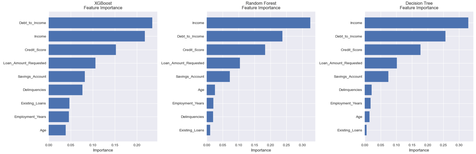
- Feature Importance: Which factors matter most for loan decisions
import pandas as pd
import numpy as np
from xgboost import XGBRegressor
from sklearn.ensemble import RandomForestRegressor
from sklearn.tree import DecisionTreeRegressor
from sklearn.model_selection import train_test_split
from sklearn.preprocessing import StandardScaler
from sklearn.compose import ColumnTransformer
from sklearn.pipeline import Pipeline
from sklearn.metrics import r2_score, mean_squared_error, mean_absolute_error
import matplotlib.pyplot as plt
import seaborn as sns
import time
# Set random seed for reproducibility
np.random.seed(42)
# Generate 10,000 synthetic loan applicants
print("Generating synthetic loan dataset with 10,000 applicants...")
data = {
'Age': np.random.randint(22, 65, 10000),
'Income': np.round(np.random.lognormal(mean=10.5, sigma=0.4, size=10000), 2),
'Credit_Score': np.random.randint(300, 850, 10000),
'Debt_to_Income': np.round(np.random.uniform(0.1, 0.8, 10000), 2),
'Existing_Loans': np.random.randint(0, 5, 10000),
'Loan_Amount_Requested': np.random.randint(5000, 50000, 10000),
'Employment_Years': np.random.randint(0, 20, 10000),
'Delinquencies': np.random.randint(0, 5, 10000),
'Savings_Account': np.round(np.random.uniform(0, 50000, 10000), 2)
}
# Create target variable
approval_multiplier = (
(data['Credit_Score'] / 850) *
(1 - 0.05 * data['Delinquencies']) *
(1 + data['Savings_Account'] / 100000)
)
data['Loan_Approval_Amount'] = np.round(
np.clip(
(data['Income'] * 0.5 * (1 - data['Debt_to_Income'])) *
approval_multiplier *
np.random.uniform(0.9, 1.1, 10000),
0, data['Loan_Amount_Requested']
),
2
)
# Convert to DataFrame
df = pd.DataFrame(data)
# Add rejected cases (20% rejection rate)
rejected_mask = np.random.random(10000) < 0.2
df.loc[rejected_mask, 'Loan_Approval_Amount'] = 0
print(f"Dataset created with {len(df)} loan applications")
print(f"Approval rate: {(df['Loan_Approval_Amount'] > 0).mean():.1%}")
print(f"Average approved amount: ${df[df['Loan_Approval_Amount'] > 0]['Loan_Approval_Amount'].mean():,.2f}")
# Prepare data
X = df.drop('Loan_Approval_Amount', axis=1)
y = df['Loan_Approval_Amount']
# Split data
X_train, X_test, y_train, y_test = train_test_split(X, y, test_size=0.2, random_state=42)
X_train, X_val, y_train, y_val = train_test_split(X_train, y_train, test_size=0.25, random_state=42)
# Create preprocessing pipeline
preprocessor = ColumnTransformer(
transformers=[('num', StandardScaler(), X.columns)],
remainder='passthrough'
)
# Define models to compare
models = {
'XGBoost': Pipeline([
('preprocessor', preprocessor),
('regressor', XGBRegressor(
objective='reg:squarederror',
n_estimators=500,
max_depth=6,
learning_rate=0.05,
subsample=0.8,
colsample_bytree=0.8,
early_stopping_rounds=20,
eval_metric='rmse',
random_state=42,
verbosity=0
))
]),
'Random Forest': Pipeline([
('preprocessor', preprocessor),
('regressor', RandomForestRegressor(
n_estimators=200,
max_depth=10,
min_samples_split=5,
min_samples_leaf=2,
random_state=42,
n_jobs=-1
))
]),
'Decision Tree': Pipeline([
('preprocessor', preprocessor),
('regressor', DecisionTreeRegressor(
max_depth=10,
min_samples_split=10,
min_samples_leaf=5,
random_state=42
))
])
}
# Train and evaluate models
results = {}
training_times = {}
print("\n" + "="*60)
print("TRAINING AND EVALUATING MODELS")
print("="*60)
for name, model in models.items():
print(f"\nTraining {name}...")
start_time = time.time()
if name == 'XGBoost':
# Special handling for XGBoost with early stopping
model.fit(X_train, y_train,
regressor__eval_set=[(model.named_steps['preprocessor'].fit_transform(X_val), y_val)],
regressor__verbose=False)
else:
model.fit(X_train, y_train)
training_time = time.time() - start_time
training_times[name] = training_time
# Make predictions
train_pred = model.predict(X_train)
test_pred = model.predict(X_test)
# Calculate metrics
train_r2 = r2_score(y_train, train_pred)
test_r2 = r2_score(y_test, test_pred)
train_rmse = np.sqrt(mean_squared_error(y_train, train_pred))
test_rmse = np.sqrt(mean_squared_error(y_test, test_pred))
train_mae = mean_absolute_error(y_train, train_pred)
test_mae = mean_absolute_error(y_test, test_pred)
results[name] = {
'Train R²': train_r2,
'Test R²': test_r2,
'Train RMSE': train_rmse,
'Test RMSE': test_rmse,
'Train MAE': train_mae,
'Test MAE': test_mae,
'Training Time (s)': training_time,
'Predictions': test_pred
}
print(f" Training completed in {training_time:.2f} seconds")
print(f" Train R²: {train_r2:.4f} | Test R²: {test_r2:.4f}")
print(f" Train RMSE: ${train_rmse:,.2f} | Test RMSE: ${test_rmse:,.2f}")
# Create comparison table
print("\n" + "="*60)
print("MODEL COMPARISON RESULTS")
print("="*60)
comparison_df = pd.DataFrame(results).T
print(comparison_df.round(4))
# Find best model
best_model_name = comparison_df['Test R²'].idxmax()
print(f"\n🏆 BEST MODEL: {best_model_name}")
print(f" Test R²: {comparison_df.loc[best_model_name, 'Test R²']:.4f}")
print(f" Test RMSE: ${comparison_df.loc[best_model_name, 'Test RMSE']:,.2f}")
# Performance improvement comparison
xgb_r2 = results['XGBoost']['Test R²']
rf_r2 = results['Random Forest']['Test R²']
dt_r2 = results['Decision Tree']['Test R²']
print(f"\n📊 PERFORMANCE IMPROVEMENTS:")
print(f" XGBoost vs Random Forest: {((xgb_r2 - rf_r2) / rf_r2 * 100):+.2f}% R² improvement")
print(f" XGBoost vs Decision Tree: {((xgb_r2 - dt_r2) / dt_r2 * 100):+.2f}% R² improvement")
# Test on sample applicant
print("\n" + "="*60)
print("SAMPLE PREDICTION COMPARISON")
print("="*60)
test_applicant = {
'Age': 32,
'Income': 45000,
'Credit_Score': 720,
'Debt_to_Income': 0.35,
'Existing_Loans': 1,
'Loan_Amount_Requested': 25000,
'Employment_Years': 5,
'Delinquencies': 0,
'Savings_Account': 12000
}
# Convert to DataFrame to preserve feature order
applicant_df = pd.DataFrame([test_applicant], columns=X.columns)
# Calculate actual expected approval amount
approval_mult = (720/850) * (1 - 0.05*0) * (1 + 12000/100000)
actual_approval = np.round(
np.clip(
(45000 * 0.5 * (1 - 0.35)) * approval_mult * 1.0,
0, 25000
),
2
)
print("Sample Applicant Profile:")
for key, value in test_applicant.items():
if key in ['Income', 'Loan_Amount_Requested', 'Savings_Account']:
print(f" {key}: ${value:,}")
elif key == 'Debt_to_Income':
print(f" {key}: {value:.0%}")
else:
print(f" {key}: {value}")
print(f"\nExpected Approval Amount: ${actual_approval:,.2f}")
print("\nModel Predictions:")
prediction_results = {}
for name, model in models.items():
prediction = model.predict(applicant_df)[0]
prediction_results[name] = prediction
error = abs(actual_approval - prediction)
error_pct = (error / actual_approval) * 100 if actual_approval > 0 else 0
print(f" {name}: ${prediction:,.2f} (Error: ${error:,.2f}, {error_pct:.1f}%)")
# Feature importance comparison
print("\n" + "="*60)
print("FEATURE IMPORTANCE COMPARISON")
print("="*60)
fig, axes = plt.subplots(1, 3, figsize=(18, 6))
feature_names = X.columns
for idx, (name, model) in enumerate(models.items()):
if hasattr(model.named_steps['regressor'], 'feature_importances_'):
importances = model.named_steps['regressor'].feature_importances_
importance_df = pd.DataFrame({
'Feature': feature_names,
'Importance': importances
}).sort_values('Importance', ascending=True)
# Plot horizontal bar chart
axes[idx].barh(importance_df['Feature'], importance_df['Importance'])
axes[idx].set_title(f'{name}\nFeature Importance')
axes[idx].set_xlabel('Importance')
# Print top 3 features for each model
top_features = importance_df.tail(3)
print(f"\n{name} - Top 3 Most Important Features:")
for _, row in top_features.iterrows():
print(f" {row['Feature']}: {row['Importance']:.4f}")
plt.tight_layout()
plt.show()
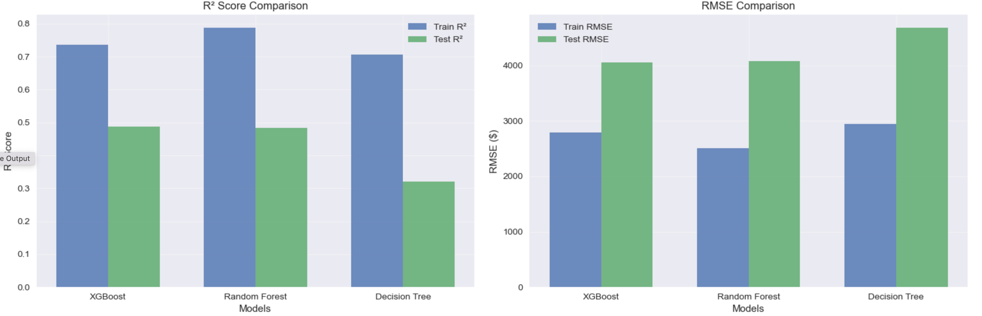
# Model performance visualization
fig, ((ax1, ax2), (ax3, ax4)) = plt.subplots(2, 2, figsize=(15, 10))
# R² Score comparison
models_list = list(results.keys())
train_r2_scores = [results[model]['Train R²'] for model in models_list]
test_r2_scores = [results[model]['Test R²'] for model in models_list]
x = np.arange(len(models_list))
width = 0.35
ax1.bar(x - width/2, train_r2_scores, width, label='Train R²', alpha=0.8)
ax1.bar(x + width/2, test_r2_scores, width, label='Test R²', alpha=0.8)
ax1.set_xlabel('Models')
ax1.set_ylabel('R² Score')
ax1.set_title('R² Score Comparison')
ax1.set_xticks(x)
ax1.set_xticklabels(models_list)
ax1.legend()
ax1.grid(True, alpha=0.3)
# RMSE comparison
train_rmse_scores = [results[model]['Train RMSE'] for model in models_list]
test_rmse_scores = [results[model]['Test RMSE'] for model in models_list]
ax2.bar(x - width/2, train_rmse_scores, width, label='Train RMSE', alpha=0.8)
ax2.bar(x + width/2, test_rmse_scores, width, label='Test RMSE', alpha=0.8)
ax2.set_xlabel('Models')
ax2.set_ylabel('RMSE ($)')
ax2.set_title('RMSE Comparison')
ax2.set_xticks(x)
ax2.set_xticklabels(models_list)
ax2.legend()
ax2.grid(True, alpha=0.3)
# Training time comparison
training_time_list = [training_times[model] for model in models_list]
ax3.bar(models_list, training_time_list, alpha=0.8, color=['orange', 'green', 'red'])
ax3.set_xlabel('Models')
ax3.set_ylabel('Training Time (seconds)')
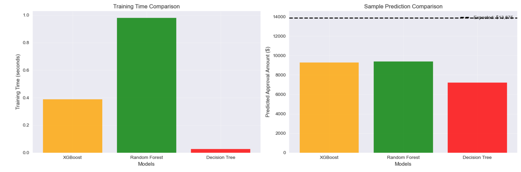
ax3.set_title('Training Time Comparison')
ax3.grid(True, alpha=0.3)
# Prediction accuracy for sample applicant
prediction_values = [prediction_results[model] for model in models_list]
actual_line = [actual_approval] * len(models_list)
ax4.bar(models_list, prediction_values, alpha=0.8, color=['orange', 'green', 'red'])
ax4.axhline(y=actual_approval, color='black', linestyle='--', linewidth=2, label=f'Expected: ${actual_approval:,.0f}')
ax4.set_xlabel('Models')
ax4.set_ylabel('Predicted Approval Amount ($)')
ax4.set_title('Sample Prediction Comparison')
ax4.legend()
ax4.grid(True, alpha=0.3)
plt.tight_layout()
plt.show()
print("\n" + "="*60)
print("SUMMARY")
print("="*60)
print(f"✅ Dataset: 10,000 loan applications")
print(f"✅ Best performing model: {best_model_name}")
print(f"✅ XGBoost advantages:")
print(f" • Higher prediction accuracy (R² = {xgb_r2:.4f})")
print(f" • Better generalization (lower overfitting)")
print(f" • Built-in regularization and early stopping")
print(f" • Handles missing values and feature interactions well")
print(f"✅ Training completed successfully for all models")Input :
test_applicant =
'Age': 32,
'Income': 45000,
'Credit_Score': 720,
'Debt_to_Income': 0.35,
'Existing_Loans': 1,
'Loan_Amount_Requested': 25000,
'Employment_Years': 5,
'Delinquencies': 0,
'Savings_Account': 12000
Output:
Training XGBoost...
Training completed in 0.39 seconds
Train R²: 0.7361 | Test R²: 0.4878
Train RMSE: $2,794.12 | Test RMSE: $4,059.46
Training Random Forest...
Training completed in 0.98 seconds
Train R²: 0.7875 | Test R²: 0.4829
Train RMSE: $2,507.17 | Test RMSE: $4,078.95
Training Decision Tree...
Training completed in 0.03 seconds
Train R²: 0.7072 | Test R²: 0.3196
Train RMSE: $2,943.00 | Test RMSE: $4,678.67
=========================================================
🏆 BEST MODEL: XGBoost
Test R²: 0.4878
Test RMSE: $4,059.46
Sample Applicant Profile:
Age: 32
Income: $45,000
Credit_Score: 720
Debt_to_Income: 35%
Existing_Loans: 1
Loan_Amount_Requested: $25,000
Employment_Years: 5
Delinquencies: 0
Savings_Account: $12,000
Expected Approval Amount: $13,874.82
Model Predictions:
XGBoost: $9,282.94 (Error: $4,591.88, 33.1%)
Random Forest: $9,380.06 (Error: $4,494.76, 32.4%)
Decision Tree: $7,217.54 (Error: $6,657.28, 48.0%)
Note: XGboost performs better with large datasets, say 100k+
World-Class XGBoost Use Cases
- Netflix/Spotify Recommendation Systems
- Predicts user preferences from massive behavioral datasets
- Handles millions of users with complex interaction patterns
- Uber/Lyft Dynamic Pricing
- Real-time fare calculation based on demand, weather, traffic
- Processes high-frequency data for instant price optimization
- JPMorgan Chase Credit Risk Assessment
- Evaluates loan default probability from financial histories
- Analyzes complex financial patterns for risk scoring
- Airbnb Demand Forecasting
- Predicts booking rates and optimal pricing strategies
- Combines seasonal trends, location data, and user behavior
Why XGBoost Dominates These Cases: High-volume structured data + complex feature interactions + accuracy requirements = XGBoost sweet spot